doi:10.4236/am.2010.15050 Published Online November 2010 (http://www.SciRP.org/journal/am)
Continuous Maps on Digital Simple Closed Curves
Laurence Boxer1,2
1Department of Computer and Information Sciences, Niagara University, New York, USA
2Department of Computer Science and Engineering, State University of New York at Buffalo, Buffalo, USA
E-mail: [email protected]
Received August 2, 2010; revised September 14, 2010; accepted September 16, 2010
Abstract
We give digital analogues of classical theorems of topology for continuous functions defined on spheres, for
digital simple closed curves. In particular, we show the following: 1) A digital simple closed curve S of
more than 4 points is not contractible, i.e., its identity map is not nullhomotopic in S; 2) Let X and Y be digital simple closed curves, each symmetric with respect to the origin, such that |Y|>5 (where |Y| is the
number of points in Y). Let f :X Y be a digitally continuous antipodal map. Then f is not nullho-
motopic in Y; 3) Let S be a digital simple closed curve that is symmetric with respect to the origin. Let
Z S
f : be a digitally continuous map. Then there is a pair of antipodes {x,x}S such that
1 | ) ( ) (
| f x f x .
Keywords:Digital Image, Digital Topology, Homotopy, Antipodal Point
1. Introduction
A digital image is a set X of lattice points that model a “continuous object” Y, where Y is a subset of a Eucli- dean space. Digital topology is concerned with deve- loping a mathematical theory of such discrete objects so that, as much as possible, digital images have topological properties that mirror those of the Euclidean objects they model; however, in digital topology we view a digital image as a graph, rather than, e.g., a metric space, as the latter would, for a finite digital image, result in a discrete topological space. Therefore, the reader is reminded that in digital topology, our “nearness” notion is the graphical notion of adjacency, rather than a neighborhood system as in classical topology; usually, we use one of the na- tural cl-adjacencies (see Section 2). Early papers in the
field, e.g., [1-8], noted that this notion of nearness allows us to express notions borrowed from classical topology, e.g., connectedness, continuous function, homotopy, and fundamental group, such that these often mirror their analogs with respect to Euclidean objects modeled by respective digital images. Applications of digital topo- logy have been found shape description and in image processing operations such as thinning and skeletoni- zation [9].
A. Rosenfeld wrote the following: “The discrete grid (of pixels or voxels) used in digital topology can be regarded as a ‘digitization’ of (two or three-dimensional)
Euclidean space; from this viewpoint, it is of interest to study conditions under which this digitization process preserves topological (or other geometric) properties” [3].
In this spirit, we obtain in this paper several properties of continuous maps on digital simple closed curves, inspired by analogs for Euclidean simple closed curves. In particular, we show that digital simple closed curves of more than 4 points are not contractible, and we obtain several results for continuous maps and antipodal points on digital simple closed curves.
2. Preliminaries
Let Z be the set of integers. Then Zd is the set of
lattice points in d-dimensional Euclidean space. Let d
Z
X and let be some adjacency relation for the members of X. Then the pair (X,) is said to be a (binary) digital image. A variety of adjacency relations are used in the study of digital images. Well known adjacencies include the following.
For a positive integer l with 1 l d and two distinct points = ( ,1 2, , ), = ( , , ,1 2 ) ,
d
d d
p p p p q q q q Z p
and q are cl-adjacent [10] if
• there are at most l indices i such that
1 |= |piqi , and
• for all other indices j such that |pjqj|1,
j
j q
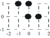
Figure 1. In Z2 , each of the points
1= (1,0)
p and
2= (0,1)
p is both c1 -adjacent and c2 -adjacent to
0= (0,0)
p , since both p1 and p2 differ from p0 by 1 in
exactly one coordinate and coincide in the other coordinate;
3= (-1,1)
p is c2-adjacent, but not c1-adjacent, to p0,
since p0 and p3 differ by 1 in both coordinates.
The notation cl is sometimes also understood as the
number of points qZd that are l
c -adjacent to a given point pZd. Thus, in Z we have =2
1
c ; in 2
Z we have c1=4 and c2=8 ; in 3
Z we have
18, = 6,
= 2
1 c
c and c3=26.
More general adjacency relations are studied in [11]. Let be an adjacency relation defined on Zd. A
-neighbor of a lattice point p is -adjacent to p. A
digital image X Zd is -connected [11] if and only
if for every pair of different points x,yX , there is a set {x0,x1,,xr} of points of a digital image X such
that x=x0,y=xr and xi and xi1 are -neighbors where i{0,1,,r1}.
Let a,bZ with a<b. A digital interval [7] is a set of the form
}. |
{ = ] ,
[a b Z zZazb
Let d0
Z
X and Y Zd1 be digital images with
0
-adjacency and 1 -adjacency respectively. A function f :X Y is said to be (0,1)-continuous [2,8], if for every 0-connected subset U of X ,
) (U
f is a 1-connected subset of Y. We say that such a function is digitally continuous.
Proposition 2.1 [2,8] Let d0
Z
X and d1
Z Y be
digital images with 0-adjacency and 1-adjacency
respectively. Then the function f :X Y is (0,1)-
continuous if and only if for every 0-adjacent points
} ,
{x0 x1 of X , either f(x0)= f(x1) or f(x0) and )
(x1
f are 1-adjacent in Y .
This characterization of continuity is what is called an
immersion, gradually varied operator, or gradually
varied mapping in [12,13].
Given digital images (Xi,i), i{0,1}, suppose there is a (0,1)-continuous bijection f :X0 X1 such that 1 0
1:X X
f is ( , )
0 1
-continuous. We say X0 and X1 are (0,1) -isomorphic [14] (this was called (0,1)-homeomorphic in [7]) and f is a
) ,
(0 1 -isomorphism (respectively, a (0,1)-homeo-
morphism).
By a digital -path from x to y in a digital image X , we mean a (2,) -continuous function
X m
f :[0, ]Z such that f(0)=x and f(m)=y .
We say m is the length of this path. A simple closed
-curve of m4 points (for some adjacencies, the minimal value of m may be greater than 4; see below) in a digital image X is a sequence { (0), (1), ,f f
( 1)}
f m of images of the -path f :[0,m1]Z
X
such that f(i) and f(j) are -adjacent if and only if j=(i1)modm . If 1
0 = } { = m
i i
x
S where
) ( = f i
xi for all i[0,m1]Z, we say the points of S
are circularly ordered.
Digital simple closed curves are often examples of digital images X Zd for which it is desirable to
consider Zd \X as a digital image with some adja-
cency (not necessarily the same adjacency as used by
X). For example, by analogy with Euclidean topology, it is desirable that a digital simple closed curve X Z2 satisfy the “Jordan curve property” of separating Z2 into two connected components (one “inside” and the other “outside” X). An example that fails to satisfy this property [10] if we allow |X |=4 is given by (X,c1), where
(0,1)} (1,1), (1,0), {(0,0), =
X
is circularly ordered, and ( \ , 2)
2 X c
Z is c2-connected. However, this anomaly is essentially due to the “small- ness” of X as a simple closed curve; it is known [1,15,16] that for m1=8 and m2=4, if
2
Z X is a digital simple closed ci-curve such that |X|mi, then
X
Z2\ has exactly 2
i
c3 -connected components, {1,2}
i . Thus, it is customary to require that a digital simple closed curve X Z2 satisfy |X|8 when
1
c- adjacency is used; |X|4 when c2-adjacency is used. Let X Zd0 and Y Zd1 be digital images with
0
-adjacency and 1 -adjacency respectively. Two )
,
(0 1 -continuous functions f,g:X Y are said to be digitally (0,1)-homotopic in Y [8] if there is a positive integer m and a function H:X[0,m]Z Y
such that
• for all xX, H(x,0)= f(x) and H(x,m)=g(x); • for all xX , the induced functionHx:[0, ]mZ
Y
defined by
, ] [0, )
, ( = )
( Z
x t H xt forall t m
H
is (2,1)-continuous; and
• for all t[0,m]Z, the induced function Ht:X Y
defined by
, )
, ( = )
(x H xt for all x X
Ht
is (0,1)-continuous.
We say that the function H is a digital (0,1)-
Additional terminology associated with homotopic maps includes the following.
• If g is a constant map, we say f is (0,1)-
nullhomotopic [8]; if, further, (X,0)=(Y,1) and
X
f =1 (the identity map on X), we say X is 0-
contractible [7,17].
• If H(x0,t)= f(x0) for some x0X and all
Z
m
t[0, ] , we say H is a (0,1)-pointed homotopy [18].
• If H:[0,m0]Z[0,m1]Z Y is a (c1,)-homotopy between (c1,)-continuous functions
Y m g
f, :[0, 0]Z such that for all t[0,m1]Z ,
(0) = (0) = )
(0,t f g
H and H(m0,t)= f(m0)= g(m0) , we say H holds the endpoints fixed [18].
Proposition 2.2 [8] Suppose f0,f1:X Y are
) ,
( -continuous and (,) -homotopic. Suppose
Z Y g
g0, 1: are (,)-continuous and (,)-ho- motopic. Then g0f0 and g1f1 are ( , ) -homo-
topic in Z.
3. Homotopy Properties of Digital Simple
Closed Curves
A classical theorem of Euclidean topology, due to L.E.J. Brouwer, states that a d-dimensional sphere Sd is not
contractible [19]. Theorem 3.3, below, is a digital analog, for d =1. We also present some related results in this section.
Proposition 3.1 Let Sa be a digital simple closed
a
-curve, a{0,1}. Let f :S0S1 be a (0,1)-
continuous function. If |S0|=|S1|, then the following
are equivalent.
a) f is one-to-one. b) f is onto.
c) f is a (0,1)-isomorphism.
Proof: Since |S0|=|S1|, the equivalence of a) and b) follows from the fact that S0 is a finite set. That c) implies both a) and b) follows from the definition of isomorphism. Therefore, we can complete the proof by showing that b) implies c).
Let 1
0 = ,}
{
= n
i i a
a x
S , where the points of Sa are circu-
larly ordered, a{0,1} . Let x1,uS1 and let
) (
= 1,
1
0,v f xu
x . Then the 1
-neighbors of x1,u in S1 are x1,(u1)modn and x1,(u1)modn, and the 0-neighbors of
v
x0, in S0 are x0,(v1)modn and x0,(v1)modn. Since f is a
continuous bijection, our choice of x0,v implies
{ 0,( 1) modv n, 0,(v 1) modn} = {
1,(u 1) modn, 1,(u 1) modn}.f x x x x
Thus,
1
1,( 1) mod 1,( 1) mod 0,( 1) mod 0,( 1) mod { u n, u n} = { v n, v n}.
f x x x x
Since u was taken as an arbitrary index, f1 is )
,
(10 -continuous, so f is a (0,1)-isomorphism.
Theorem 3.2 Let S be a simple closed -curve
and let H:S[0,m]Z S be a (,) -homotopy
between an isomorphism H0 and Hm= ,f where
S S
f( ) . Then |S|=4.
Proof: Let 1
0 = } { = n
i i x
S , where the points of S are circularly ordered.
There exists w[1,m]Z such that
}. ) ( | ] [0, { min
= t m H S S
w Z t
Without loss of generality, x1Hw(S). Then the induced function Hw1 is a bijection, so there exists
S
xu such that H(xu,w1)=x1. By Proposition 3.1, }
, { = }) ,
({ ( 1)mod ( 1)mod 0 2
1 x x x x
Hw u n u n , and the continuity
property of homotopy implies H(xu,w){x0,x2} . Without loss of generality,
(u 1) modn, 1 =
0H x w x (1) and
u,
= 2.H x w x (2)
Suppose n>4. Equation (2) implies }
, , { ) ,
(x( 1)mod w x1 x2 x3
H u n , but this is impossible, for
the following reasons.
• H(x(u1)modn,w)x1, by choice of x1.
• H(x(u1)modn,w){x2,x3}, from Equation (1), because 4
>
n implies neither x2 nor x3 is -adjacent to x0. The contradiction arose from the assumption that
4 >
n . Therefore, we must have n4. Since a digital simple closed curve is assumed to have at least 4 points, we must have n=4.
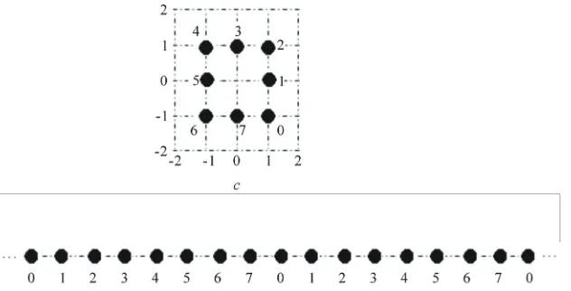
In [8], an example is given of a simple closed c2- curve SZ2 such that Z2\S has 2
1
c -connected components, with |S|=4, such that S is c2-contrac- tible (see Figure 2). By contrast, we have the following.
Theorem 3.3 Let (S,) be a simple closed -curve such that |S|>4. Then S is not -contractible.
Proof: It follows from Theorem 3.2 that if |S|>4, then there cannot be a (,)-homotopy between 1S
and a constant map in S.
It is natural to ask whether we can obtain an analog of Theorem 3.3 for higher dimensions. In order to do so, we must decide what is an appropriate digital model for the
k -dimensional Euclidean sphere Sk . The literature
contains the following.
• Let X2k be the set of all points k Z
p such that
p is a c1-neighbor of the origin.
Then ([10], Proposition 4.1) X2k is ck-contractible.
Notice that this example generalizes the contractibility of a 4-point digital simple closed curve [8] (see Figure 2 for the planar version); the contractibility seems due to the smallness of the image, rather than its form.
• Let BdIk denote the boundary of a digital k-cube, i.e., for some integer n>2,
1
= {( , , ) [0, 1] | {1, , }, {0, 1}}.
k
k k Z
i
Bd I x x n for some i k
x n
Figure 2. c2-contraction of X4, a digital simple closed c2-curve, via H : X4×[0,2]ZX4. (a) shows X4. Points are
labeled by indices. We have H x( ,0) =x for all x X 4. Arrows show the “motion” of x x2, 3 at the next step. (b) shows the
results of the first step of the contraction: H x( ,1) =0 H(x3,1) =x0; H x( ,1)1 = H x( ,1)2 = x1. The arrow shows the motion at
the next step of the contraction. (c) shows the results of the final step of the contraction: H x ,( i 2)= x0 for all i{0,1,2,3}.
See Figure 3 for the planar version. Then ([7], Coro- llary 5.9) for n> 2, Bd Ik is not c1-contractible.
The next result may be interpreted as stating that for 4
>
n , a map homotopic to 1S must be a “rotation” of
the points of S.
Theorem 3.4 Let S be a simple closed -curve such that |S|=n>4. Let f :SS be a (,) -
continuous function such that f is (,)-homotopic
to 1S. Then, for some integer j , we have
. 1] [0, =
)
(xi x(i j)modn foralli n Z
f
Proof: Let H:S[0,m]Z S be a (,)-homo-
topy from 1S to f . For t[0,m]Z , let Ht:SS
be the induced map. The assertion follows from the following.
Claim 1: For each t[0,m]Z, there is an integer j
such that Ht(xi)= x(ij)modn for all i[0,n1]Z.
To prove Claim 1, we argue by mathematical induc- tion on t. For t=0, we can clearly take j=0. Now, suppose the claim is valid for t[0,u]Z such that
m u<
0 . Then, in particular, there is an integer j
such that Hu(xi)=x(ij)modn for all i[0,n1]Z. The
continuity properties of homotopy imply Hu1( )x0 ( 1) mod ( 1) mod
{xj n, ,x xj j n}.
Without loss of generality, Hu1(x0)=xj. This is the
initial case of the following:
Claim 2: Hu1(xk)=x(kj)modn for all k[0,n1]Z.
Suppose the equation of Claim 2 is true for all
Z v
k[0, ] , for some v[0,n2]Z. In particular,
. =
)
( ( )mod
1 v v j n
u x x
H (3)
By the continuity properties of homotopy, Hu1(xv1) is adjacent to or coincides with Hu1(xv)=x(vj)modn and with
1 ( 1 ) mod
( ) = .
u v v j n
H x x Thus, Hu1(xv1) { x(v j ) modn,
(v 1 j) modn}
x . Since Hu1 must also be an isomorphism by Theorem 3.2, from Equation (3), Hu1(xv1) =
(v1 j) modn
x . This completes the induction proof for the Claim 2, which, in turn, completes the induction proof for the Claim 1. Thus, the assertion is established.
4. Antipodal Maps
A classical theorem of Euclidean topology, due to K. Borsuk, states that a continuous antipodal map :f Sd
d S
from the d-dimensional unit sphere to itself is not homotopic to a constant map [19]. In this section, we obtain a digital analog, Theorem 4.16, for d=1.
We say a set X Zd is symmetric with respect to the origin if X satisfies the property that
.
X x if only and if X
x
Suppose we have X Zd0, YZd1, and X is sym-
metric with respect to the origin. A function f X: Y
is called antipodal-preserving or an
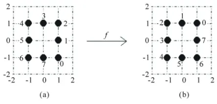
[image:4.595.381.483.525.697.2]Figure 4. A digital simple closed c1-curve
7 =0 = { }i i
S x and a
1 1
( , )c c -continuous map f S: S such that f is ( , )c c1 1
-homotopic to 1S. According to Theorem 3.4, such a map
f must “rotate” the members of S. In (a), points of S are labeled by indices. In (b), each y S is labeled by the index of the point xiS such that f x( ) =i y. Here, we
have f x( ) =i x( 2) mod 8i for all i.
antipodal map if f(x)=f(x) for all xX [19]. In this section, we study properties of continuous antipodal maps between digital simple closed curves.
Lemma 4.1 Let p0,p1 be cl-adjacent points in d Z , d
l
1 . Then p0 and p1 are not antipodal.
Proof: The hypothesis implies that there is an index i
such that p0 and p1 differ by 1 in the
th
i coordinate: 1
|=
|p0,ip1,i . If p0 and p1 are antipodal, this would imply {p0,i,p1,i}={1/2,1/2}, which is impossible.
Lemma 4.2 Let p0,p1 be cl-adjacent points in d
Z ,
d l
1 . Then p0 and p1 are cl-adjacent.
Proof: Elementary, and left to the reader.
Lemma 4.3 Let 1
0 = } { = n
i i x
S be a digital simple closed
l
c -curve in Z such that the points of S are cir- d
cularly ordered. If S is symmetric with respect to the origin, then the origin is not a member of S .
Proof: Suppose the origin is a member of S. Without
loss of generality, x0 is the origin, and therefore is its own antipode.
By Lemma 4.2, x1 and xn1 are antipodes; by Lemma 4.1, these points are not cl -adjacent. This
establishes the base case of an induction argument: 1 1 = 1 0 =
1={xi}i {xn j}j
S is a connected subset of S, such that x1 and xn1 are non-adjacent antipodes; hence,
1
S is (cl,c1)-isomorphic to a digital interval. Now, suppose for some integer k , 1k<(n1)/2 ,
k j j n k i i
k x x
S ={ }=0{ }=1 is (cl,c1)-isomorphic to a digital interval, with endpoints xk and xnk, such that xm
and xnm are non-adjacent antipodes for all
} , {1, k
m . Then, by Lemma 4.2, xk1 and xnk1 are antipodes, and by Lemma 4.1, these points are not
l
c -adjacent. Thus, 1
1 = 1
0 =
1={ } { }
k j j n k i i
k x x
S is (cl,c1)-
isomorphic to a digital interval, with endpoints x1 and
1
n
x .
This completes an induction argument from which we conclude that 1 1)/2 ( = 1)/2 ( 0 = { } } { = n n n i i n i i x x S
is (cl,c1)-isomorphic to a digital arc, with the endpoints of S being x(n1)/2 and xn(n1)/2 , such that
( 1)/2
1 i n implies xi and xni are non-adjacent
antipodes.
• If n is odd, then n1 is even, so S=S. This is a contradiction, since S is not a simple closed cl-
curve.
• If n is even, then S=S\{xn/2}. Since S is symmetric with respect to the origin, we must have that
/2
n
x is the origin. But since S is a simple closed
l
c -curve in which x0 is the origin, this is a contra- diction.
Whether n is even or odd, the assumption that the origin belongs to S yields a contradiction. Hence, the origin is not a member of S.
Lemma 4.4 Let 1
0 = } { = n
i i x
S be a digital simple closed
l
c -curve in Z such that the points of S are d
circularly ordered. If S is symmetric with respect to the origin, then n is even.
Proof: By Lemma 4.3, the origin is not a member of
S, so every member of S is distinct from its antipode. Therefore, n must be even.
Lemma 4.5 Let 1
0 = } { = n
i i x
S be a digital simple closed
l
c -curve in Z such that the points of S are cir- d
cularly ordered. If S is symmetric with respect to the origin, then for all i we have xi =x(in/2)modn.
Proof: Suppose there is a simple closed cl-curve
1 0 = } { = n
i i x
S that is symmetric with respect to the origin such that the points of S are circularly ordered, such that there exist indices u,v such that xu and xv are
antipodes and v(un/2)modn . Without loss of generality, we can assume u=0, vn/2.
Then, from Lemma 4.2, x1 is antipodal to either xv1 or x(v1)modn. Without loss of generality, x1 and xv1 are antipodal. If v1=1, this is a contradiction of Lemma 4.3; or, if v1=2, this is a contradiction of Lemma 4.1; otherwise, we inductively repeat the argument above with the antipodal (by Lemma 4.2) pair
) ,
(x2 xv2 , etc., until similarly we obtain a contradiction of Lemma 4.3 or of Lemma 4.1. The assertion follows.
We have the following.
Theorem 4.6 Let di
i Z
S be simple closed
i
-curves, i{0,1}, each symmetric with respect to the
origin. Let f :S0S1 be a (0,1) -continuous
antipodal map. Then f is onto.
Proof: Let 1
0 =
1={ }
n i i x
podal, it follows from Lemma 4.5 that f(p)=xn/2. Since f is continuous and S0 is 0-connected, it follows that one of the 1-paths in S1 from x0 to
/2
n
x is contained in f(S0). Without loss of generality, ) ( } { 0 /2 0
= f S
x n
j
j . For n/2< j<n, there exists qS0 such that f(q)=xjn/2, and from Lemma 4.5,
/ 2
0 = = ( )
= ( ) ( ) ( ).
j j n
x x f q
since f is antipodal f q f S
Thus, f(S0)=S1.
Corollary 4.7 Let di
i Z
S be simple closed i-
curves, i{0,1}, each symmetric with respect to the origin. Let f :S0S1 be a (0,1)-continuous anti- podal map. If |S0|=|S1|, then f is a (,) -iso- morphism.
Proof: By Theorem 4.6, f is onto. The assertion follows from Proposition 3.1.
Proposition 4.8 Let 1
0 = } { = nX
i i x
X be a simple closed
X
-curve with circularly ordered points. LetY =
1 =0
{ }yi inY
be a simple closed Y-curve with circularly
ordered points. Suppose H:X[0,m]Z Y is a
) ,
(X Y -homotopy between the (X,Y)-continuous
maps H0,Hm such that H0(x0)=Hm(x0). Then there is a (X,Y)-homotopyG X: [0, ]mZ Y between
0
H and Hm such thatG x t( , ) =0 H x0( )0 for all
Z m t[0, ]
Proof: Without loss of generality, H0(x0)= y0. Let
Z
Z m
m
a:[0, ] [0, ] be defined by a(t)=i if
i y t x
H( 0, )= .
Let G:X[0,m]Z Y be defined by
. = ) , ( , = ) ,
(xi t y[ja(t)]modnY if H xi t yj
G
Roughly, we may think of G(xi,t) as rotating )
, (x t
H i counter to the rotation of H(x0,t), so that the image under G of x0 at time t is constant with respect to t. We show below that G is a homotopy. In particular, a(0)=a(m)=0 , so G0 =H0 and
m
m H
G = ; and, for all t[0,m]Z,
0 [ ( ) ( )]mod 0
( , ) = a t a t nY = .
G x t y y
For each xiX and t[0,m]Z , if Ht(xi)= yj
then we have the following.
• By the continuity of Ht, we have
( 1) mod ( 1) mod ( 1) mod ( 1) mod
({ , }) { , , }.
t i nX i nX j nY j j nY
H x x y y y
Therefore, G xt( ) =i y[j a t ( )]modnY and
1 mod 1 mod
1 mod mod 1 mod
,
, , .
t i nX i nX
j a t nY j a t nY j a t nY
G x x
y y y
Therefore, Gt is (X,Y)-continuous.
• Let Gxi:[0,m]Z Y be the induced function de-
fined by Gxi(t)=G(xi,t). To simplify the following, let
1 0
( 1) = ( ) = ( ),
xi i i
G H x H x 1
( 1) = ( ) = ( ),
xi m i m i
G m H x H x
1) ( = ) ( = 0 = (0) = 1)
( a a m a m
a . Note that the con-
tinuity of Hx0 implies that
{ (a t1), (a t1)} { ( ) 1, ( ), ( ) 1}. a t a t a t
Suppose Ht(xi)= yj, so G txi( ) =y[j a t ( )]modnY.
If a(t1)=a(t)1, then
[ ( 1)]mod [ ( ) 1]mod
( 1) = =
xi j a t nY j a t nY
G t y y is Y-adjacent
to ( )
xi
G t .
If a(t1)=a(t), then Gxi(t1)=Gxi(t). If a(t1)=a(t)1, then
[ ( 1)]mod [ ( ) 1]mod
( 1) = =
xi j a t nY j a t nY
G t y y is Y-adjacent
to Gxi(t).
Similarly, 1)Gxi(t is Y-adjacent to, or equal to, ( ).
xi
G t Therefore, the induced function Gxi is (c1,Y)-
continuous.
Therefore, G is a homotopy between H0 and Hm
such that G(x0,t)=H0(x0) for all t[0,m]Z.
Let (X,X) and (Y,Y) be digital images and let
Y
y . We denote by y X: Y (or, for short, y) the constant map y x( ) =y for all xX .
Lemma 4.9 Let (X,X) and (Y,Y) be digital
simple closed curves and let f :X Y be (X,Y)-
homotopic to a constant map. Then for any x0X,
)) ( , ( ) , (
: X x0 Y f x0
f is (X,Y)-pointed homotopic
to the constant map f(x0).
Proof: Let F:X[0,m0]Z Y be a (X,Y) -
homotopy between f and the constant map y0 for some y0Y . Since Y is Y -connected, there is a
path p:[0,m1]Z Y from y0 to f(x0). Then the map H:X[0,m0m1]Z Y defined by
, ) ( ; 0 ) , ( = ) , ( 1 0 0 0 0 m m t m if m t p m t if t x F t x H
is a homotopy between f and f(x0). The assertion
follows from Proposition 4.8.
Given a digital image (X,) and a positive integer
n, for xX we define [20]
( , ) = { }
{ |
}.
N x n x
y X there is a path in X from y to x of length at most n
The covering space and the lifting of maps are notions borrowed from algebraic topology that have been important in digital algebraic topology. We have the following.
Definition 4.10 [20] Let (E,E) and (B,B) be
digital images. Let p:EB be a (E,B) -conti-
nuous function. Suppose for each bB there exists
N
• for some N and some index set M ,
); ( )
, ( = )) , (
( 1
1
b p e with e
N b
N
p B iM E i i
• if i,jM, i j, then
( , )=
) ,
(
E ei N E ej
N ; and
• the restriction map p|NE(ei,):NE(ei,)NB(b,)
is a (E,B)-isomorphism for all iM .
Then the map p is a (E,B) - covering map, and
the pair (E,p) is a (E,B) - covering (or covering
space).
The following is a somewhat simpler characterization of the digital covering than given in Definition 4.10.
Theorem 4.11 [14] Let (E,E) and (B,B) be
digital images. Let p:EB be a (E,B) -
continuous function. Then the map p is a (E,B)-
covering map if and only if for each bB, there is an
index set M such that
• 1( ( ,1))= ( ,1) i E M i
B b N e
N
p
, with e p 1(b)
i
;
• if i,jM, i j, then NE(ei,1)NE(ej,1)=;
and
• the restriction map p|NE(ei,1):NE(ei,1)NB(b,1)
is a (E,B)-isomorphism for all iM .
The following is a minor generalization of an example of a digital covering map given in [20].
Example 4.12 Let m d
i
i Z
c C 1
0 =
} {
= be a circularly
ordered simple closed -curve. Let p:ZC be
defined by p(z)=zmodm for all zZ. Then p is a (c1,)-covering map (see Figure 5).
Definition 4.13 [20] For digital images (E,E), )
,
(BB , and (X,X), let p:EB be a (E,B)
covering map, and let f :X B be (X,B) -
continuous. A lifting of f with respect to p is a
) ,
(X E -continuous function F:X E such that
f F p = .
See Figure 6 for an illustration of Definition 4.13. Theorem 4.14 [20] Let (E,E) be a digital image
and e0E . Let (B,B) be a digital image and
B
b0 . Let p:EB be a (E,B)-covering map
such that p(e0)=b0. Then a B-path f :[0,m]Z B beginning at b0 has a unique lifting with respect to p
to a path ~f in E starting at e0.
For a positive integer n, a (E,B)-covering map
B E
p: is called a radius n local isomorphism [21] if for each bB and ep b1( ),
( , ) |N e n
E
p
( , )
B
N b n
is an isomorphism. It was observed in [14] that every covering is a radius 1 local isomorphism, but there are coverings that are not radius 2 local isomor- phisms.
Theorem 4.15 [21] Let (E,E) be a digital image
and e0E . Let (B,B) be a digital image and
B
b0 . Let p:EB be a (E,B)-covering map
such that p(e0)=b0. Suppose p is a radius 2 local
isomorphism. For E-paths g0,g1:[0,m]Z E that
start at e0, if there is a B-homotopy in B from
0
g
p to pg1 that holds the endpoints fixed, then
) ( = )
( 1
0 m g m
g , and there is a E-homotopy in E
from g0 to g1 that holds the endpoints fixed.
Theorem 4.16 Let 1
0 = } { = nX
i i x
X be a simple closed
X
-curve with points circularly ordered, that is
symmetric with respect to the origin. Let 1
0 = } { = nY
i i y
Y be
a simple closed Y-curve with points circularly ordered, that is symmetric with respect to the origin. Let
Y X
f : be a (X,Y)-continuous antipodal map. If
5 |>
|Y , then f is not (0,1)-nullhomotopic.
Proof: Suppose there is such a function f that
is (0,1) -nullhomotopic. From Lemma 4.9, f is
point- ed homotopic to f(x0).
Let b:[0,nX]Z X be defined by b(t)= xtmodnX.
Let p:ZY be the (c1,Y)-covering map defined
by p(z)= yzmodnY (see Example 4.12). By Proposition
2.2, f b and f(x0)b are (c1,Y)-homotopic paths
[image:7.595.145.461.532.693.2]in Y . From Theorem 4.14, these functions have unique
Figure 5. A simple closed c1-curve C and a covering by the digital line Z. Members of C are labeled by their respective
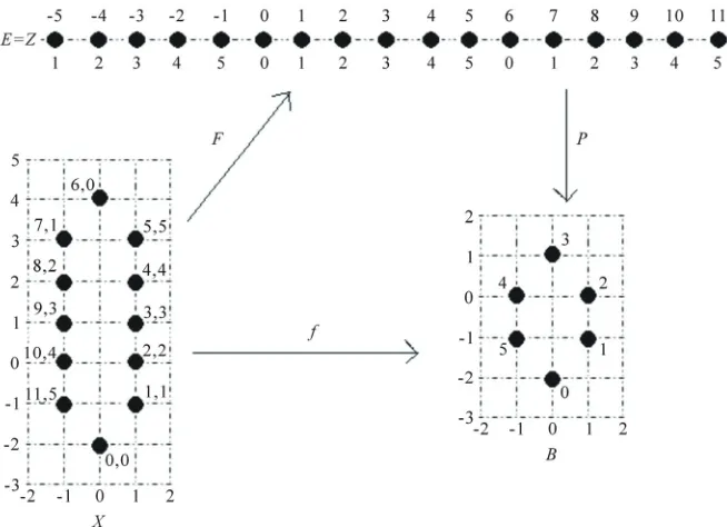
Figure 6. Example of lifting. 5 =0 = { }i i
B b is a simple closed c2-curve whose members are labeled by their indices. E=Z has
its points z labeled above by their coordinates and labeled below by the index i such that p z( ) =bi (note p is given by
the formula p z( ) =bzmod 6).
11 =0 = { }m m
X x is a simple closed c2-curve that has points labeled by a pair m n, such that m is
the index of the point, f x( ) =m bn (thus, f is defined by f x( ) =m bmmod 6), and F x( ) =m m. Since p is a covering map (by
Example 4.12) and p F = f , F is a lifting of f with respect to p.
liftings with respect to p to paths F0 and F1 , respectively, in Z , each starting at 0p1(f(b(0))). Since |Y|>5, NY(f(x0),2)Y , so p is a radius 2
local isomorphism. From Theorem 4.15, F0 and F1 must end at the same point. Indeed, this point must be 0, for the uniqueness of F1 implies F1 must be the cons- tant map 0.
Since f is an antipodal map, we must have
. 1] /2 [0, /2
= | ) ( /2) (
|F0 tnX F0 t nY forallt nX Z (4)
Since F0(0)=0, F0(nX/2){nY/2,nY/2}. Without
loss of generality,
/2. = /2) (
0 nX nY
F (5) Since F is continuous and nY >5, a simple induc-
tion argument based on Equations (4) and (5) shows that
) ( > /2)
( 0
0 t n F t
F X for all t[0,nX/21]Z. But since 0
= ) (
0 nX
F , this implies with Equation (4) that
/2 = /2) (
0 nX nY
F , which contradicts Equation (5). The assertion follows from the contradiction.
5. Antipodes Mapped Together
A classical result of topology is that if f is a conti- nuous map from the d-dimensional unit sphere Sd to
Euclidean d-space Rd, then there is a pair of antipodes
d
S x
x, such that f(x)= f(x) [17]. For d=1, the following is a digital analog.
Theorem 5.1 Let S be a digital simple closed
l
c-curve with 1
0 =
} {
= n
i i
x
S , where the points of S are
circularly ordered. Suppose S is symmetric with
respect to the origin. Suppose f :SZ is a (cl,c1)- continuous function. Then there is a pair of antipodes
S x
x, such that | f(x) f(x)|1.
Proof: By Lemma 4.4, n is even. Consider the
function g:[0,n1]Z Z defined byg i( ) = ( )f xi
( /2) mod ( i n n)
f x . By Lemma 4.5, we are done if, for some
i, g(i)=0. Therefore, we assume for all i that
0. ) (i
g (6) Clearly, for all i,
). ( = ] mod /2)
[(i n n g i
g (7) The continuity of f implies that
2. | 1) ( ) (
|g i g i (8) It follows from Equation (7) that g takes both posi- tive and negative values, so from inequality (6), there is an index j such that g(j) and g(j1) have oppo- site sign; without loss of generality, g(j)>0 and
0 < 1) (j
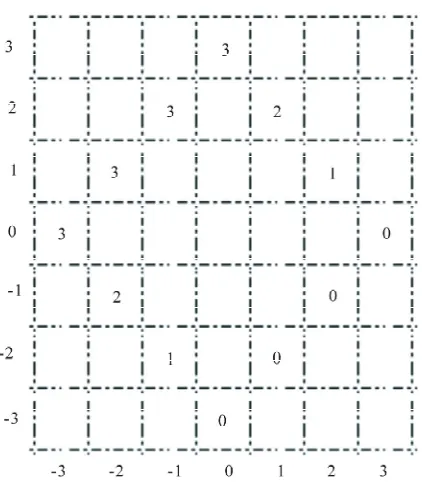
Figure 7. S and f S: Z. Each number in the grid labels a point of S, showing the image of the grid point under f . Note for s0= (1,2), | ( )f s0 f(s0) |= 1, but
there is no s S for which f s( ) = ( )f s .
1 = ) (j
g , and the assertion follows.
Theorem 5.1 parallels, in a sense, a result of [2]: In the Euclidean line, a continuous function mapping an interval to itself has a fixed point; in the digital world, a (c1,c1)-
continuous function f :[a,b]Z [a,b]Z has a “near-
fixed” point, i.e., a point x such that |x f(x)|1. That we cannot, in general, conclude the existence of antipodes mapped to the same point in Theorem 5.1, is illustrated in the following example (note the simple closed curve has more than 4 points). Let S= {( , ) | | | | |= 3}x y x y . Then S is a simple closed c2- curve in Z2. The function f :SZ given by
3, = (0,3) = 1,2) ( = 2,1) ( = 3,0)
( f f f
f
2, = (1,2) = 1) 2,
( f
f
1, = (2,1) = 2) 1,
( f
f
0, = (3,0) = 1) (2, = 2) (1, = 3)
(0, f f f
f
is a (c2,c1)-continuous function such that f x( ) f(x) 0
for each xS. See Figure 7.
6. Further Remarks
In this paper, we have obtained several analogs of classical theorems of Euclidean topology concerning maps on digital simple closed curves. We have shown
that digital simple closed curves of more than 4 points are not contractible; that a continuous antipodal map from a digital simple closed curve to itself is not nullhomotopic; and that a continuous map from a digital simple closed curve to the digital line must map a pair of antipodes within 1 of each other. Except as indicated concerning whether or not a digital model of a sphere is contractible, it is not known at the current writing whether these results extend to higher dimensional digital models of Euclidean spheres.
We thank the anonymous referees for their helpful suggestions.
7. References
[1] A. Rosenfeld, “Digital Topology,” American Mathe- matical Monthly, Vol. 86, 1979, pp. 76-87.
[2] A. Rosenfeld, “Continuous Functions on Digital Pic- tures,” Pattern Recognition Letters, Vol. 4, No. 3, 1986, pp. 177-184.
[3] A. Rosenfeld, “Directions in Digital Topology,” 11th Summer Conference on General Topology and Applica- tions, 1995. http://atlas-conferences.com/cgi-bin/abstract/ caaf-71
[4] Q. F. Stout, “Topological Matching,” Proceedings 15th Annual Symposium on Theory of Computing, Boston, 1983, pp. 24-31.
[5] T. Y. Kong, “A Digital Fundamental Group,” Computers and Graphics, Vol. 13, No. 1, 1989, pp. 159-166. [6] T. Y. Kong, A. W. Roscoe and A. Rosenfeld, “Concepts
of Digital Topology,” Topology and Its Applications, Vol. 46, No. 3, 1992, pp. 219-262.
[7] L. Boxer, “Digitally Continuous Functions,” Pattern Recognition Letters, Vol. 15, No. 8, 1994, pp. 833-839. [8] L. Boxer, “A Classical Construction for the Digital
Fundamental Group,” Journal of Mathematical Imaging and Vision, Vol. 10, No. 1, 1999, pp. 51-62.
[9] T. Y. Kong and A. Rosenfeld, “Topological Algorithms for Digital Image Processing,” Elsevier, New York, 1996. [10] L. Boxer, “Homotopy Properties of Sphere-Like Digital Images,” Journal of Mathematical Imaging and Vision, Vol. 24, No. 2, 2006, pp. 167-175.
[11] G. T. Herman, “Oriented Surfaces in Digital Spaces,” CVGIP: Graphical Models and Image Processing, Vol. 55, No. 1, 1993, pp. 381-396.
[12] L. Chen, “Gradually Varied Surfaces and Its Optimal Uniform Approximation,” SPIE Proceedings, Bellingham, Vol. 2182 1994, pp. 300-307.
[13] L. Chen, “Discrete Surfaces and Manifolds,” Scientific Practical Computing, Rockville, 2004.
[14] L. Boxer, “Digital Products, Wedges, and Covering Spaces,” Journal of Mathematical Imaging and Vision, Vol. 25, 2006, pp. 159-171.
Current Topics in Pattern Recognition Research, Research Trends, Council of Scientific Information, 1994. http://cosmic.rrz.uni-hamburg.de/webcat/mathematik/eck hardt/eck00001/eck00001.pdf
[16] R. O. Duda, P. E. Hart and J. H. Munson, “Graphical Data Processing Research Study and Experimental Investigation,” Descriptive Note: Quarterly Report No. 7, March 1967, pp. 28-30.
[17] E. Khalimsky, “Motion, Deformation, and Homotopy in Finite Spaces,” Proceedings IEEE International Confer- ence on Systems, Man, and Cybernetics, Boston, 1987, pp. 227-234.
[18] L. Boxer, “Properties of Digital Homotopy,” Journal of Mathematical Imaging and Vision, Vol. 22, No. 1, 2005, pp. 19-26.
[19] J. Dugundji, “Topology,” Allyn and Bacon, Inc., Boston, 1966.
[20] S. E. Han, “Non-Product Property of the Digital Funda- mental Group,” Information Sciences, Vol. 171, No. 1-3, 2005, pp. 73-91.
![Figure 2. 2results of the first step of the contraction: c -contraction of X , a digital simple closed 4c2 -curve, via H : X4×[0,2]ZX](https://thumb-us.123doks.com/thumbv2/123dok_us/8990983.395934/4.595.381.483.525.697/figure-results-contraction-contraction-digital-simple-closed-curve.webp)