Abstract—Calcium, a vital second messenger for signal transduction in neurons, plays an important role in almost every organ of our human body. Thus modeling of Calcium signaling mechanism can help us understand this mechanism in a better way. Here, a finite element mathematical model has been developed to study the flow of calcium in two dimensions with time. This model assumes EBA (Excess Buffering Approximation), incorporating all the important parameters like time, association rate, influx, buffer concentration, diffusion coefficient etc. Finite element method is used to obtain calcium concentration in two dimensions and numerical integration is used to compute the effect of time over 2–D Calcium profile. Comparative study of calcium signaling in two dimensions with time is done with important physiological parameters, like buffer concentration, buffer association rate. A program has been developed for the entire problem and simulated on an AMD-Turion 64X2 machine to compute the numerical results.
Index Terms— FEM, EBA, MATLAB, Ca2+ influx, Ca2+ profile.
I. INTRODUCTION
Neurons communicate to each other through two types of junctions or synapses, namely, i) Electrical synapse and ii) Chemical synapse. The communication through electrical synapse is fast while the communication through chemical synapse is slow. However, chemical synapses are considered to be more significant than electrical synapses as they come into play when the distance between the neurons is more than 4 – 5 nm [1]. When the gap in between neurons is more, i.e. of the order of 20 – 50 nm, then signaling in between neurons cannot take place through electrical synapses. In such cases, electrical signal is converted into a chemical signal so that the message can be transmitted through a chemical synapse. This process of conversion of an electrical signal into a chemical signal is known as the process of signal transduction. Calcium acts as a switch in this process of signal transduction and decides whether a particular electrical signal is to be converted into a chemical signal or not. This Ca2+ is also known to regulate a number of other cellular functions like secretion, fertilization, gene expression, muscle contraction [2], [3], [4]. When an electrical signal arrives near the end point of an axon (cytosol), it causes the Voltage Dependent Calcium Channels (VDCC) to open which facilitates the inflow of extracellular Ca2+ inside the cytosol. This inflow of Ca2+ creates transient domains of high intracellular Ca2+
Manuscript received April 10, 2009.
S. G. Tewari is with the Department of Allied Sciences & Management, Asia Pacific Institute of Information Technology, Panipat, Haryana 132103 INDIA (phone: 91-9425727127; fax: 91-180-2577273; e-mail: [email protected]).
K. R. Pardasani is with the Department of Mathematics, Maulana Azad National Institute of Technology, Bhopal, MP 462051 INDIA (e-mail: [email protected]).
concentration near the VDCC [5]. Near to these VDCC’s there are neurotransmitters filled synaptic vesicles to which cytosolic Ca2+ gets bound to initiate the process of exocytosis [6]. Since, exocytosis occurs in the immediate vicinity of VDCC’s therefore, [Ca2+]i transients cannot be measured in
situ due to the spatiotemporal limitations of the [Ca2+]i
measuring technologies [7]. Mathematical and Computational simulation of Ca2+ kinetics provides a beautiful alternative to study the effect of several parameters over [Ca2+]i transients [8], [5], [9].
In this article, Ca2+ dynamics are studied by developing a Finite Element Model for two–dimensional unsteady state Ca2+ diffusion under EBA. A computer program has been developed in MATLAB for the whole approach and simulated on an AMD Turion 64X2 machine with 1.6 GHz processing speed and 2.5 GB memory. The numerical results are used to demonstrate the two–dimensional Ca2+ profile in x and y directions. Also, numerical results are used to study the interrelationship between [Ca2+]i and other parameters viz.
buffer specie, buffer concentration, association rate etc. II. MATHEMATICAL FORMULATION
Calcium kinetics in neurons is governed by a set of reaction-diffusion equations which can be framed assuming the following bimolecular reaction between Ca2+ and buffer species:
2
[ ] [ ] [ ]
k
j j
k
Ca B CaB
+ −
+ + ⇌ (1)
where [Bj] and [CaBj] are free and bound buffer respectively,
and ‘j’ is an index over buffer species. It is conventional to assume isotropy, homogeneity and Fickian diffusion. With these assumptions, Ca2+ dynamics can be represented with the help of the following system of partial differential equations [5], [8], [9]:
2 2 2 2 2
2 2
[ ] [ ] [ ]
( )
Ca j
j
Ca Ca Ca
D R
t x y
r
σδ
+ + +
∂ = ∂ +∂ +
∂ ∂ ∂
+
∑
(2)2 2
2 2
[ ] [ ] [ ]
j
j j j
B j
B B B
D R
t x y
∂ ∂ ∂
= + +
∂ ∂ ∂ (3)
2 2
2 2
[ ] [ ] [ ]
j
j j j
CaB j
CaB CaB CaB
D R
t x y
∂ ∂ ∂
= + −
∂ ∂ ∂ (4)
where,
2
[ ][ ] [ ]
j j j j j
R = −k+ B Ca + +k CaB− (5) DCa, DBj, DCaBj are diffusion coefficient of free calcium, free
buffer, and bound buffer, respectively; kj+ and kj− are
Finite Element Model to Study Two Dimensional
Unsteady State Cytosolic Calcium Diffusion
in Presence of Excess Buffers
Shivendra G. Tewari and K. R. Pardasani
IAENG International Journal of Applied Mathematics, 40:3, IJAM_40_3_01
association and dissociation rate constants for buffer ‘j’, respectively and δ( )r is the standard Dirac delta function placed at the Ca2+ source. For stationary, immobile buffers or fixed buffers DBj = DCaBj = 0. The first term on the right hand
side of (2) comes as a result of Fick’s law of diffusion, the second term Rj is known as the reaction term and the third
term is the source amplitude due to the calcium channel. If we assume a single mobile buffer specie, i.e. [Bj] = [B] and make
two more assumptions i) Excess Buffer Approximation (EBA), due to Neher [8], i.e. the buffer concentration is present in excess and ii) Buffer is constant in space and time, i.e. [B] = [CaB] = constant, then (2 – 5) can be simplified to,
(
)
2 2 2 2 2
2 2 2 [ ] [ ] [ ] [ ] [ ] [ ] ( ) Ca m
Ca Ca Ca
D
t x y
k B Ca Ca σδ r
+ + + + + ∞ ∞ ∂ = ∂ +∂ ∂ ∂ ∂ − − + (6)
where, [B]∞ and [Ca]∞ are steady state buffer and calcium concentration respectively.
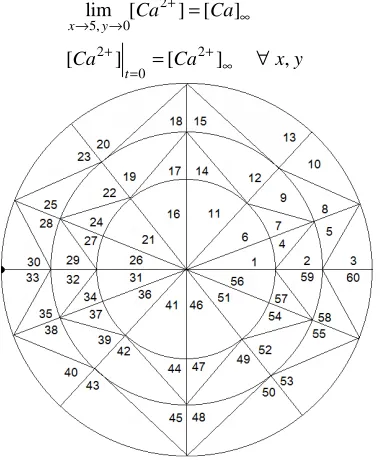
In this article, we have considered cytosol to be a circle of radius 5 µm. The centre of the circle is supposed to be situated at origin (i.e. x = 0, y = 0). We have assumed that there is a point source of calcium situated at x= −5,y=0. An appropriate flux condition for it can be framed as [5], [9],
2 5, 0 [ ] lim Ca x y Ca D x σ + →− → ∂ − = ∂ (7)
For other boundary condition and initial condition, it is assumed that [Ca2+] attains its steady state concentration of 0.1 µM as it goes far away from the source i.e.
2
5, 0
2 2
0
lim [ ] [ ]
[ ] [ ] ,
x y
t
Ca Ca
Ca Ca x y
+ ∞ → → + + ∞ = =
= ∀ (8)
Fig. 1 Finite Element discretization of the cytosol, small black circle at element number ‘30’ and ‘33’ represents point source of calcium.
Further, the cytosol is divided into 60 linear triangular elements of different sizes (see Fig. 1).
The discretized variational form of (6 – 8) can be written as:
( ) ( )2
( ) ( )2 ( )2
2 2 ( ) ( ) ( ) ( ) 2 1 2 1 2 + 2 e e
e e e
x y A e e e e Ca Ca A A u u u
I u u dA
u u
dA u dA
D t D
λ λ σ µ ∞ ∂ = + + − ∂ − ∂
∫∫
∫∫
∫
(9)Here, we have used ‘u’ in lieu of [Ca2+] for notational convenience, e = 1(1)60, λis the characteristic length and is equal to
[ ] Ca
m D
k+ B∞ , the subscripts ‘x’ and ‘y’ denote derivatives of ‘u’ in respective directions. Also the second term (µ( )e =1) for e = 30, 33 and (µ( )e =0) for rest of the
elements. The shape function of concentration variation within each element is defined by [10],
( ) ( ) ( ) ( ) ( )
( ) ( )
( , ) ( , ) ( , )
( , )
e e e e e
i i j j
e e
k k
u x y N x y u N x y u N x y u
= +
+ (10)
where, ( )e , ( )e, ( )e i j k
u u u are element nodal Ca2+ concentrations and ( ) ( ) ( )
, ,
e e e i j k
N N N are element shape functions given by,
( ) ( ) ( ) ( ) ( ) ( ) ( ) ( ) ( ) ( ) ( ) ( ) ( ) ( ) ( ) 1 ( , ) ( ) 2 1 ( , ) ( ) 2 1 ( , ) ( ) 2
e e e e
i e i i i
e e e e
j e j j j
e e e e
k e k k k
N x y a b x c y
A
N x y a b x c y
A
N x y a b x c y
A
= + +
= + +
= + +
(11)
Here, ‘A( )e ’ is the area of the element and ( ) ( ) ( )
, , ,
e e e i j k
a a a
( ) ( ) ( ) ( ) ( ) ( )
, , , , ,
e e e e e e i j k i j k
b b b c c c are,
( ) ( ) ( ) ( ) ( ) ( ) ( ) ( ) ( ) e
i j k k j e
j k i i k e
k i j j i e
i j k
e
j k i
e
k i j
e
i k j
e
j i k
e
k j i
a x y x y
a x y x y
a x y x y
b y y
b y y
b y y
c x x
c x x
c x x
= − = − = − = − = − = − = − = − = − (12)
Now, using (10 – 12) in (9) and extremizing (9) with respect to nodal concentration we have,
( ) ( ) ( ) ( ) ( ) ( ) ( ) ( ) 2 ( ) ( ) ( ) ( ) ( ) ( ) 2 1 ( ) 1 T T
e e e e
e x x y y
e T e e i A e T e e Ca A e e e Ca A A
N N N N
I
u dA
u N N
u
N N dA
D t
N u
dA N dA
D λ σ µ λ ∞ ∂ + ∂ = ∂ + ∂ + ∂ − −
∫∫
∫∫
∫∫
∫
(13)Here, u( )e =ui uj ukT. Assembling (13) for e = 1(1)60, we have,
60 ( )
1
0 e
i e i
I I
u = u
∂ = ∂ =
∂
∑
∂ (14)where, i = 1, 2, …, 37. Rearranging (14) and writing in matrix form, we have a system of ordinary differential equations (see Appendix for details),
IAENG International Journal of Applied Mathematics, 40:3, IJAM_40_3_01
[image:2.595.76.271.410.640.2][ ]
37 37 37 1[ ]
37 37[ ]
37 1 37 1x x x x
x u
K u M F
t
∂
+ =
∂
(15)
here, u = u1, u2, …, u37, [K] and [M] are system matrices, and
[F] is the system vector. For the solution of (15), we have developed a computer program in MATLAB that uses numerical integration to approximate the solution at discrete time steps [11]. The time taken for simulating the mathematical model for 1 sec, while taking ∆ =t 0.0001sec, is nearly 2 minutes on the aforesaid computer.
[image:3.595.310.535.128.318.2]III. NUMERICAL RESULTS AND DISCUSSION In this section, numerical results are shown in the form of figures explaining the relationship observed between the physiological parameters. All the investigations were done assuming that cytosolic Ca2+ is buffered using 50 µM EGTA, Table I List of physiological parameters used for numerical results [12], [5], [13],
Symbol Parameter Value
DCa Diffusion coefficient 250 µm2 . s-1
km+ (EGTA) Buffer association rate 1.5 µM-1.s-1
km+ (BAPTA) Buffer association rate 600 µM-1.s-1
km+
(Troponin-C)
Buffer association rate 90 µM-1.s-1
km+
(Calmodulin-D28K)
Buffer association rate 250 µM-1.s-1
[Bm]∞ Buffer concentration 50 µM
[Ca2+]∞ Background Ca2+ Concentration
0.1 µM
σ
Source amplitude 1 pAF Faraday’s Constant 96487 C/moles
V Volume of the cytosol 523.6 µm3 *All parameter values are taken as per Table I unless otherwise stated.
Here source amplitude is converted into µM.s-1 by using Faradays constant and using the fact that 1 L = 1015 µm3 to compute the results.
In Fig. 2, cytosolic diffusion is shown in x and y directions for time t = 100 ms. As proposed Ca2+ attains its background concentration of 0.1 µM as it goes far away from the Ca2+ channel. Since source amplitude is taken to be 1 pA therefore the highest Ca2+ concentration observed is 1176 µM. Thus, if an electrical signal arrives at the mouth of a VDCC, it can increase the intracellular Ca2+ concentration to an extent of 1176 µM. As observed by Brose et al. [14], synaptotagmin is activated at high cytosolic [Ca2+] ~ 10 µM and not at lower Ca2+ concentrations. An ample amount of neurotransmitters are supposed be released and thus signal transduction can take place at this point of time. In Fig. 3, the effect of time over two-dimensional calcium profile is shown. In this figure changes with respect to time are observed for whole of the cytosol. It is apparent from the figure that calcium begins to
rise slowly as time elapses and attains a steady state calcium concentration of 1176 µM. It was also observed that there is no change in calcium profile after 100 ms (not shown in this article) which means that calcium attains steady state after 100 ms.
[image:3.595.47.291.279.540.2]Fig. 2 Calcium diffusion in x and y directions for time, t = 100ms.
Fig. 3 Effect of increasing time over 2–D Ca2+ profile.
Fig. 4 Effect of increasing buffer concentration on two dimensional calcium profile.
Fig. 4 shows the effect of increasing buffer concentration for
IAENG International Journal of Applied Mathematics, 40:3, IJAM_40_3_01
[image:3.595.311.546.368.534.2] [image:3.595.311.545.564.731.2]time t = 100 ms. Fig. 4(A), 4(B), 4(C) and 4(D) are for buffer concentration taken to be 50 µM, 100 µM, 150 µM, and 200
µM, respectively. In all the four cases buffer specie is taken to be Ethylene Glycol - bis(beta – aminoethyl - ether)-N,N,N',N'-TetraAcetate(EGTA). As expected the increase in buffer concentration increases the decay of calcium which is evident in both the directions. In other words, it can be said that increase in buffer concentration alters the time required to achieve the steady state.
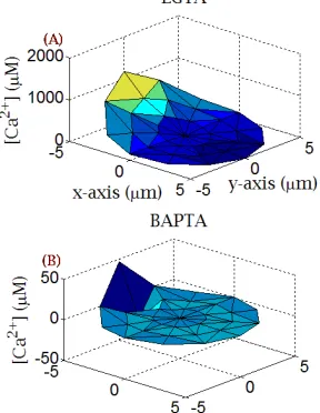
In Fig. 5, the effect of two diverse calcium chelators on cytosolic calcium profile is shown. These chelators are used to increase or decrease the time required by calcium to attain steady state.
[image:4.595.61.205.218.404.2]We used two exogenous buffers i) BAPTA (1,2-bis(o-minophenoxy)ethane-N,N,N’,N’-tetraacetic acid) which is a very fast calcium chelator and ii) EGTA which is a very slow calcium chelator. It is observed from the figure that the highest calcium concentration is only 46.37 µM (see Fig. 5(B)) when cytosol is introduced to BAPTA while the same is about 1176 µM (see Fig. 5(A)) when cytosol is introduced to EGTA. It is so because when we introduce BAPTA inside the cytosol it binds calcium faster as compared to EGTA and reduces the free calcium concentration faster than EGTA.
Fig. 6 Effect of different buffer types over 1–D Ca2+ profile.
In Fig. 6 Ca2+ diffusion in x-direction is shown, for different buffer types, just as if we are studying Ca2+ diffusion in one-dimension. Because of the presence of different buffer types there is a variation in cytosolic Ca2+ profile. Thus, before plotting the curves the [Ca2+] values were normalized to make them comparable. To be specific, Ca2+ diffusion was studied for three different buffer types namely, i) EGTA, ii) Troponin-C and iii) Calmodulin-D28K. The solid curve is for
Ca2+ diffusion in the presence of 50 µM EGTA, the ‘*’ curve is for Ca2+ diffusion in the presence of 50 µM Troponin-C and the ‘o’ curve is for Ca2+ diffusion in the presence of 50
µM Calmodulin-D28K. These results further validate our
previous hypothesis, as for the given three buffers λvalues are decreasing and hence the time to achieve steady state is also decreasing. It can also be concluded from the figure that the time to achieve steady state is directly proportional to characteristic length constant ‘λ ’. As, this characteristic length constant ‘λ’ depends upon association rate and buffer concentration.
IV. CONCLUSION
The results shown in this paper are primarily for Ca2+ diffusion in 2-D with relevance to buffers following EBA. Further, the results obtained in this paper are in agreement with the physiological facts. Some of the results obtained have also been observed by previous researchers but they were all for one–dimensional case. The finite element model developed is quite versatile and flexible as we are able to incorporate the minute details of processes involved and study the effect of excess buffers on calcium diffusion in cytosol. There is a significant variation in calcium profiles due to various excess buffers used in the present problem. Further, the results obtained can be of great use to biomedical scientists for development of new protocols for treatment and diagnosis of neuronal diseases.
APPENDIX When we extremize (9) we have,
( ) ( ) ( ) ( )
( ) ( ) ( ) ( )
2 2
( ) ( )
( ) ( )
1
e e e e
i i
e e e e
i A i i
e e
Ca i e e
Ca i A
u u u u
x u x y u y
u
I u u u
dA
u u u
u u
D u t
u dA
D u
λ λ
σ µ
∞
∂
∂ ∂ ∂ ∂ ∂ ∂
+
∂ ∂ ∂ ∂ ∂ ∂
∂ = + ∂ − ∂
∂ ∂ ∂
∂ ∂
+
∂ ∂
∂ −
∂
∫∫
∫
(16)
Also from (10) we have,
( )
( )
( )
( )
e
j e
i k
e
i i
e i i
N
N N
u
u
x x x x
N u
u x x
u N u
∂
∂ ∂
∂ =
∂ ∂ ∂ ∂
∂
∂ ∂ =
∂ ∂ ∂
∂ =
∂
(17) Fig. 5 Change in calcium profile for two calcium
chelators namely EGTA and BAPTA.
IAENG International Journal of Applied Mathematics, 40:3, IJAM_40_3_01
[image:4.595.59.290.585.754.2][ ]
( )e T
j
i u k
u u
u N
t t t t
∂
∂ ∂
∂ =
∂ ∂ ∂ ∂ (18)
where,
[ ]
N =Ni Nj Nk. Thus, (16) can be written as,( )
( ) ( ) ( ) ( ) ( ) 0
e
e e e e e
i I
K u M u F
u
∂ = + − =
∂ ɺ (19)
where uɺ represents time derivative of ‘u’ and K(e), M(e), F(e) are given by,
( ) ( ) ( ) ( )
( )
( ) ( ) 2
1
( )
e e T e e T
e
e e T A
N N N N
x x y y
K dA
N N
λ
∂ ∂ ∂ ∂
+
∂ ∂ ∂ ∂
=
+
∫∫
(20)( ) ( ) ( )
( ) ( ) ( ) ( )
2
1
e e e T
Ca A
e e e e
Ca
A A
M N N dA
D
u
F N dA N dA
D
σ µ
λ∞ ∂
=
= +
∫∫
∫∫
∫
(21)
Further from (11) we have, N
b x N
c y
α α
α α
∂ = ∂ ∂ =
∂
(22)
where, α =i j k, , . Also, since our triangle is linear by using factorial formula we have [16],
2
( ) ( )
2 ( )
2
2
( ) ( )
2 ( )
2
( ) ( ) ( )
( ) ( )
1 4
1 4
2 1 1
1 2 1
12
1 1 2
1 3
i i j i k e e T
i j j k j e
A
i k j k k
i i j i k e e T
i j j k j e
A
i k j k k
e e e T
A
e e
A
b b b b b
N N
dA b b b b b
x x A
b b b b b c c c c c
N N
dA c c c c c
y y A
c c c c c
A N N dA
A N dA
∂ ∂ =
∂ ∂
∂ ∂ =
∂ ∂
=
=
∫∫
∫∫
∫∫
∫∫
11
(23)
For the assembly of all the elements, we write,
36
( ) ( ) ( )
1
36
( ) ( ) ( )
1
36
( ) ( )
1
e e e T e
e e e T e
e e e
K D K D
M D M D
F D F
=
=
=
=
=
=
∑
∑
∑
(24)
where,
( )
0 0 0
1 0 0
0 1 0
0 0 1
0 0 0
th
e th
th i row
D j row
k row
=
⋮ ⋮ ⋮
⋮ ⋮ ⋮
(25)
Thus for the whole system we have,
[ ]
37 37 37 1[ ]
37 37[ ]
37 137 1
x x x x
x u
K u M F
t
∂
+ =
∂
ACKNOWLEDGMENT
The authors are highly grateful to Department of Biotechnology, New Delhi, India for providing support in the form of Bioinformatics Infrastructure Facility for carrying out this work.
REFERENCES
[1] E. R. Kandel, J. H. Schwartz, and T. M. Jessell, “Principles of Neural Science”, 4th ed. McGraw-Hill, New York, 2000.
[2] G. Ramadori, F. Moriconi, I. Malik, and J. Dudas, “Physiology and Pathophysiology of Liver inflammation, damage and repair”, Journal of physiology and pharmacology, 59, 2008, pp. 107 – 117.
[3] L. Sun et al., “Ca2+ Homeostasis Regulates Xenopus Oocyte maturation”, Biology Of Reproduction, 78, 2008, pp. 726–735.\ [4] S. Rüdiger, J. Shuai, W. Huisinga, C. Nagaiah, G. Warnecke, I. Parker,
and M. Falcke, “Hybrid Stochastic and Deterministic Simulations of Calcium Blips”, Biophysical J. 93, 2007, pp. 1847-1857.
[5] G.D. Smith, “Analytical Steady-State Solution to the rapid buffering approximation near an open Ca2+ channel”. Biophys. J. 71, 1996, pp. 3064-3072.
[6] K. Broadie, H. J. Bellen, A. Di Antonio, J. T. Littleton, and T. L. Schwarz, “Absence of synaptotagmin disrupts excitation-secretion coupling during synaptic transmission”, Proc. Nat. Acad. Sci. USA, 91, 1994, pp. 10727-10731.
[7] Y. Tang, T. Schlumpberger, T. Kim, M. Lueker, and R. S. Zucker, “Effects of Mobile Buffers on Facilitation: Experimental and Computational Studies”. Biophys. J., 78, 2000, pp. 2735–2751. [8] E. Neher, “Concentration profiles of intracellular Ca2+ in the presence
of diffusible chelator”, Exp. Brain Res. Ser. 14, 1986, pp. 80-96. [9] G. D. Smith, L. Dai, R. M. Miura, and A. Sherman, “Asymptotic
Analysis of buffered Ca2+ diffusion near a point source”, SIAM J. of Applied of Math. 61, 2000, pp. 1816-1838.
[10] S. S. Rao, “The Finite Element Method in engineering”, Elsevier Science and Technology books, 2004.
[11] Y.W. Kwon, and H. Bang, “The Finite Element Method using MATLAB”, CRC Press, London, 1997.
[12] N. L. Allbritton, T. Meyer, and L. Stryer, “Range of messenger action of calcium ion and inositol 1,4,5-trisphosphate”. Science. 258, 1992, pp. 1812–1815.
[13] G. D. Smith, J. Wagner, and J. Keizer, “Validity of the rapid buffering approximation near a point source of Ca2+ ions”. Biophys. J. 70(6), 1996, pp. 2527-2539.
[14] N. Brose, A. G. Petrenko, T.C. Sudhof, and R. Jahn, “Synaptotagmin: a calcium sensor on the synaptic vesicle surface”, Science, 256, 1992, pp. 1021-1025.
[15] G. L. Fain, “Moleculer and cellular physiology of neurons”. Prentice Hall of India, 2005.
[16] L. J. Segerlind, “Applied Finite Element Analysis”, John Wiley and Sons, New York, 1984.
![Table I List of physiological parameters used for numerical results [12], [5], [13],](https://thumb-us.123doks.com/thumbv2/123dok_us/387808.536303/3.595.47.291.279.540/table-i-list-physiological-parameters-used-numerical-results.webp)