A Methodology for Selection of an Optimum Gear Ratio for Single Speed Gearbox coupled with Continuously Variable Transmission to Achieve Best Acceleration Performance

©IJRASET: All Rights are Reserved

116

A Methodology for Selection of an Optimum Gear

Ratio for Single Speed Gearbox coupled with

Continuously Variable Transmission to Achieve

Best Acceleration Performance

1, 2, 3

Department of Mechanical Engineering, Vishwakarma Institute of Technology

4

Department of Mechanical Engineering, Vishwakarma University, Pune, India

Abstract: The work presented deals with a numerical iterative methodology that was implemented to find an optimum speed ratio for a gearbox coupled with continuously variable transmission (CVT). The optimization has been done with the primary design objective of maximizing acceleration performance of an SAE Baja Vehicle. The time taken by the vehicle to traverse a certain specified distance is a function of the gear ratio of the vehicle. An initial estimate of this gear ratio was computed based on analytical calculations considering weight shift due to acceleration for a no-tire-slip condition. However, this analytical computation ignores the additional tractive effort afforded by moment of aerodynamic drag force and loss of torque due to rotational inertia of transmission components. Hence, this computation results in under-utilization of the available tractive effort and a more aggressive gear ratio is possible without the loss of traction. This optimized ratio is not possible to be computed manually, hence an algorithm has been developed for iterative calculations. Along with aerodynamic drag, rolling resistance, tire slip and engine rev limitations along with various system efficiencies have been considered in the program. The program computes the kinetic parameters in four distinct phases of the CVT. This algorithm predicts a more aggressive ratio which can be implemented without loss of traction. Measuring the performance improvement achieved in terms of 150 ft. traversal time, an 8.54% improvement was observed compared to the analytically predicted gear ratio.

Keywords: Continuously Variable Transmission, SAE Baja, Acceleration Performance, Traversal Time, MATLAB, tire slip.

I. INTRODUCTION

The motivation behind this work was to develop an optimized transmission system for an SAE Baja Vehicle. The metric used for determining vehicle performance is the 150 ft. straight line traversal time, wherein the minimum time suggests the best transmission system. Numerical simulation has been a preferred method for determining vehicle characteristics such as fuel economy and performance. One such vehicle simulation tool for automobiles and light commercial vehicles is VEHSIM [3]. A simplified algorithm has been derived by using the analytical treatment done by Zub R. W., to determine the optimum speed ratio for a single speed transmission system coupled to a centrifugal Continuously Variable Transmission, a common layout for SAE Baja vehicles.

II. DESIGNAPPROACH

To achieve the best possible acceleration performance, one needs to first estimate the normal force acting on the driving wheels. In this particular case discussed in the paper, the vehicle is rear wheel driven and is assumed to be accelerating on level ground without any hitch forces pulling back on the vehicle. This normal force is a function of the acceleration of the vehicle due to the dynamic effects of weight transfer between the axles. Hence, an additional equation relating the acceleration of the vehicle and normal force is required. For maximizing the acceleration performance, the entire traction available at the driving wheels must be utilized. Using these two conditions the normal reaction at the rear wheels is calculated. This normal reaction is used to calculate the available tractive force. Given the available torque at the engine, the available tractive force is equated to the tractive effort of the engine in terms of a gear ratio. Solution of this equation is the first estimate of the gear ratio required to achieve maximum acceleration performance.

©IJRASET: All Rights are Reserved

117

transmission ratio due to upshifting etc. need to be considered. This gives rise to constantly changing tractive effort and resistive forces which is beyond the limits of manual calculations. Hence a numerical approach is preferred, where in a short time step is considered during which all the kinematic parameters and dynamic parameters can be held constant. During this short time step, the various resistive forces acting on the vehicle and the tractive effort provided by the engine can be calculated. This data is used to calculate the acceleration, velocity and displacement of the vehicle for that particular time step. These kinematic parameters are then again fed back to calculate the resistive and tractive forces for next time step. Following is the schematic which illustrates the process flow:

Fig. 1 Process Flowchart

This numerical integration can be continued until the required length of trajectory has been traversed. Summation of all the number of time steps required gives the total traversal time, which can be plotted as a function of the input gear ratio. The most optimum gear ratio is the one which gives minimum possible traversal time for the specified vehicle parameters.

III. ANALYTICALTREATMENT

A. Estimation Of Available Tractive Force

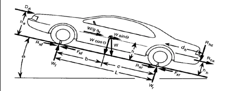
The normal reaction at the rear wheel calculated by considering a free body diagram of the vehicle shown in fig. 2. The notations used in the analysis are as follows.

©IJRASET: All Rights are Reserved

118

W- weight of the vehicle b – Distance of center of gravity from front axle

W/g.ax- d’Alembert Force c - Distance of center of gravity from rear axle

Wf and Wr - Dynamic weights carried by front and rear wheels. L – Wheel base

Fxf and Fxr – Tractive forces on front and rear wheel h – Height of center of gravity from ground

Rxf and Rxr – Rolling resistance forces on front and rear wheel respectively ha – Height of center of aerodynamic force from ground

DA – Aerodynamic drag force hh – Height of hitch point from ground

Rhz and Rhx – Vertical and longitudinal hitch forces dh – Distance of hitch point from rear axle

θ - Grade angle

Considering summation of torques about point B (assuming zero angular acceleration of vehicle in pitch), the following equation is obtained.

( cos ( ) W _A sin ) /

W _r Wb R_{hx h}h R_hz d_hL  _g a h_x D h_aWh  L (1)

For a vehicle accelerating at low speed on level ground without any hitch forces the equation reduces to

(b ax h)

W _rW _L _{g L} (2)

For maximum possible acceleration, the entire traction at the driving wheels is used to push the vehicle. Hence the following equation is obtained.

(max) Wr

a_x  _W g (3)

Where, µ is the coefficient of static friction at the road-tire interface and g is the gravitational acceleration of earth (9.81 m/s2).

Solving equations (2) and (3) simultaneously the following equation is obtained.

Wb W

r  Lh (4)

Thus, the available tractive force at rear wheels is given by

( )

xr available

Wb F

L h

 _



 (5)

B. Analytical Calculations For Estimating Initial Gear Ratio

Now, considering the tractive effort of the engine at the driving wheels in terms of gear ratio, following equation can be derived.

T N_{e tf tf}

xr r

F   (6)

Where,

Te – Torque provided by the engine ηtf – Final driveline efficiency

Ntf – Final driveline gear ratio r – Radius of wheel

Equation (6) ignores the effect of rotational inertia of transmission components and wheels. However, this effect has been considered in the algorithm of the code.

Equating equation (5) and (6), the final driveline gear ratio can be expressed as

( )

rWb N

tf T_{e tf} l h 

 



©IJRASET: All Rights are Reserved

119

The final driveline ratio consists of the CVT reduction times the gear ratio of the two-step compound single-speed gearbox coupled to it. The CVT used in this study is Gaged GX9 having a low speed ratio of 3.9:1 and an overdrive speed ratio of 0.9. During the shifting phase, this ratio varies continuously. Substituting the speed reduction obtained from CVT in equation (7), the following expression is obtained.

( )

gearbox

CVT

rWb

N _{N T l h}

e tf 

 



 (8)

Substituting the vehicle parameters in equation (8), the gearbox ratio evaluated for this specific vehicle is 7.23. This gear ratio is a close approximation of the optimum gear ratio. However, it tends to underutilize the available ground traction. This is owing to that fact that the effect of aerodynamic drag and rotational inertia of wheels and transmission components has not been considered.

IV. NUMERICALITERATIVEMETHODOLOGYUSEDFOROPTIMIZATION

To refine the initial estimation of the gear ratio, a numerical algorithm has been developed. This algorithm considers a very small time step (0.001 seconds for this study/5 to 6 million calculations per simulation) during which the traction and resistive forces acting on the vehicle and the associated acceleration can be assumed to be constant. This value was iteratively selected for achieving a reasonable computational accuracy and acceptable simulation run time. The vehicle velocity at the start of this time step and the computed acceleration for that time step can then be used to calculate the vehicle velocity at the end of the time step by applying elementary equations of kinematic motion. Also, the displacement of the vehicle during this time step can be calculated.

v v_i a t_ts

f   (9)

2 1 2

ts v_it a t_ts

s

where,

vf – Final vehicle velocity at the end of the time step ats – Constant vehicle acceleration during the time step

vi – Initial vehicle velocity at the start of the time step t – Duration of the time step

sts – Displacement of the vehicle during the time step

This computed final vehicle velocity can then be fed back into the algorithm to calculate the tractive and resistive forces experienced by the vehicle for the next time step.

For this particular case, the only resistive forces acting on the vehicle are the aerodynamic drag for (DA) and the rolling resistance offered by tires (Rx). The expressions for all these forces have been stated below.

2 1 2

A D

D





V C A

x xf xr r

R



R



R



f W

Where,

ρ – Density of air at normal temperature and pressure CD – Coefficient of aerodynamic drag

V – Vehicle velocity fr– Coefficient of rolling resistance

The coefficient of aerodynamic drag has been considered to be 0.7 in this case. For typical SAE Baja vehicles, this coefficient varies from 0.6-1 [4], [5]. Considering the range of speeds experience by such a vehicle, the rolling resistance can be safely assumed to be constant. The coefficient of rolling resistance for tractor travelling on hard muddy terrain has been used in the simulation [1] Using this data, the algorithm computes the resistive forces on the vehicle at each time step.

©IJRASET: All Rights are Reserved

120

2 2

[( ) ]

2

T N_{e tf tf ax}

I I N I N I

x r e t tf d f w _r

F       (13)

Where,

Ie – Rotational inertial of engine Id – Rotational inertia of driveshaft

It – Rotational inertia of transmission Iw – Rotational inertia of wheels and axle shafts

Nf– Numerical ratio final drive ratio

In this equation the tires are assumed to be in pure rolling. For the vehicle under consideration, the engine output torque is the net torque provided by the engine considering inertial losses. Hence the term Ie refers only to the rotational inertia of the primary CVT pulley. The term It refers to the rotational inertial of the secondary CVT pulley, gears and shafts inside the gearbox. A final drive system is also absent in the vehicle as provisions for transmitting power to the half shafts is included in the gearbox itself [6]. Hence, Id = 0.

Also, by applying Newton’s Second Law (NSL) of motion

Ma F D R

x  x A x (14)

Combining equation (13) and (14), longitudinal vehicle acceleration can be expressed as follows.

2

{( ) }

2

T N_{e tf tf}

D_A R_x

r a

x

I_e I_t N_tf I_w

M

r



 



 _{ } 

 _ 

 

 

(15)

Computation of tractive forces is comparatively more complex than that of resistive forces. Firstly, the variation of engine torque at wide-open throttle with revving speed of the engine needs to be accounted for in the algorithm. The engine used for the vehicle is Briggs and Stratton M19H. The following graph shows the torque variation of this engine.

Figure 3: Briggs and Stratton M19H net torque curve (Courtesy: Briggs & Stratton Racing, Milwaukee, WI)

For modelling this variation mathematically, a quadratic least square regression of the data has been used to relate the torque output of the engine at any given engine speed. This equation has been expressed below.

-6 2 -3

-1.4879 10

8.3945 10

7.8578

T





N





N



Where,

T – Torque delivered by engine at wide open throttle (N-m) N – Engine speed in revolutions per minute (RPM)

©IJRASET: All Rights are Reserved

121

Figure 4: Speed diagram of variable speed transmission [2]

The mathematical modelling of these phases in the algorithm has been expressed below.

A. CVT Pre-engagement Phase (Clutching Phase)

During this phase, there is belt slippage occurring at the primary sheave of the CVT which provides the clutching action required to start the vehicle from standstill. Numerical analysis of this phase involves complex kinematical modelling of the components of primary clutch such as roller-cam interface and dynamics of belt-sheave interactions [10], [11], [12]. Such a mathematical treatment is out of scope for this work and hence the following assumptions have been considered for modelling of the clutching phase. Firstly, the engine speed is assumed to be a quadratic spline variation in terms of vehicle velocity. The equation for this variation can be derived from the following boundary conditions.

0

V

 

N



N

e e

V



V



N



N

0

0

dN

dV



Where,

Ve – Speed of the vehicle at 100% primary clutch engagement Ne – Speed of engine at 100% primary clutch engagement

Ni – Idling speed of engine

The value of Ve can be analytically determined by gearing calculations. The value of Ni and Ne are selected for required vehicle performance. The engine idling speed for the vehicle under study is set to 1600 RPM by adjusting the throttle valve opening and the required engagement speed is set to 1800 RPM by adjusting the preloaded tension of the primary spring.

Thus, the variation of engine speed with respect to vehicle velocity during this phase can be expressed as

2

60.7370

1600.0000

N



V



©IJRASET: All Rights are Reserved

122

The power delivered by the engine during the clutching phase is lost in the form of frictional heat generated due to belt slipping. Hence, only a fraction of the torque produced by the engine as given by equation (16) is transmitted to the wheels. The torque transmitted by the primary sheave is directly proportional to the centrifugal force acting on the flyweights. Hence the torque during this phase has been assumed to vary quadratically with engine speed. The equation for this variation is given by the following boundary conditions.

i i

N



N



T



T

e e

N



N



T



T

1 e

N N

dT

C

dN



Where,

Ti – Theoretical net initial torque generated by engine at Ni C1 – Slope of torque curve at Ne

Te – Net torque generated by engine at Ne

Te and C2 can be computed by substituting N = Ne in equation (16) and its first order differential respectively. Ti can be approximated by considering the side pressure exerted by the primary sheave onto the V-belt [7] [8] [9]. Thus, the equation for torque provided by engine during this phase is given by

-4 2

-1.5568 10

0.5634 - 491.6480

T





N



N

The above assumptions also consider the efficiency of power transmission of the CVT during the clutching phase. Hence, the only the transmission efficiency of the gearbox [13] and CV joints [14] has been considered. Also, if wheel slip occurs during the clutching phase, it is assumed that the clutching effect of the CVT stops as power flows through the path of minimum resistance, which now occurs at the road-wheel interface. In this case, the torque is calculated using equation (16)

Substituting equation (24) in equation (15), the acceleration of the vehicle during this phase can be calculated. This acceleration is assumed to be constant during any time step and is used to calculate the velocities at the end of the time step using equation (9). In this phase the initial velocity of the vehicle is zero. The final velocity achieved at the end of the time step is then substituted in equation (20) to re-calculate the engine RPM for the next phase. Also, the displacement of the vehicle at each time step is calculated using equation (10). These iterations are continued till the CVT is 100% engage and no macro slippage of belt occurs.

B. Constant Speed Ratio Phases (N V )

After completing of the clutching phase, the engine speed varies linearly with vehicle velocity. Hence, there exists a fixed constant gearing ratio between the engine and the wheels. This relationship can be expressed mathematically using the following equation.

2

60

2

N

N

V

C V

r







The constant of proportionality C2 is different for the low ratio and the high ratio of CVT due to different overall final drive ratio. An approximation of the system efficiency in these phases needs to make to accurately predict the acceleration performance. The efficiency variation has been given in [2] and shown in following graph.

©IJRASET: All Rights are Reserved

123

Considering a CVT efficiency of 85% during this phase, the overall system efficiency can be obtained. The acceleration in this phase can be calculated by using equation (15) and (16). The final velocity of the vehicle from the previous phase is used as the initial velocity for this phase. For each time step, the final velocity obtained from equation (9) is used to calculate the engine speed for the next time step using equation (25). The algorithm computes the vehicle performance sequentially as the final kinematic parameters obtained from the simulation are inputs for the next. Hence, the simulation of the low ratio phase of CVT is done immediately after the clutching phase. This phase ends when the engine speed reaches maximum peak power (shift point). The simulation of the overdrive phase (high ratio) can be performed only after the shifting phase has been completed. The high ratio phase also considers the engine maximum revving limitations and stops accelerating the vehicle in case such high engine speeds are reached.

C. CVT Shifting Phase

When the engine reaches peak power, the function of the CVT is to maintain the engine at this speed by changing the overall gearing ratio. By keeping the engine in the maximum power regime of its power curve, the performance of the vehicle can be maximized. This constancy of engine speed is achieved by means of changing the CVT speed ratio, thereby affecting the overall gearing ratio. As the vehicle speeds up, the CVT up-shifts, thereby not allowing the engine speed to increase with the wheel speed. Assuming perfect shift curve, this change in the CVT speed ratio can be mathematically expressed by the following equation.

2 1 60 rNs N_CVT N V gearbox   (26)

Where Ns is the engine speed at which the CVT shift occurs. This speed is determined by the flyweight masses of the primary spring and the torsion spring stiffness of the secondary pulley spring. Another factor affecting the shifting response of the CVT are the cam profiles used in both the pulleys. For this vehicle, the CVT has been tuned to shift at engine speed of 3600 RPM. Efficiency of the CVT has been assumed to be 90% during this phase (see fig. 5).

Similar to the other phase, acceleration and velocities for each time step are computed using the equations discussed previously. The velocity obtained at the end of each time step is used to back calculate the changed CVT ratio using equation (26). This simulation phase is continued till the CVT reaches its overdrive ratio.

D. Case Of Insufficient Traction

During all of these phases of the CVT simulation, only the power limited performance of the vehicle has been considered. In order to ensure the validity of the simulation, the accelerations obtained at each time step need to be compared with the traction limited acceleration possible at the time step. The traction limited acceleration can be obtained by modifying equation (2) to include the moment of aerodynamic drag forces.

( ) D hA a

L

a b x h

W _rW _L _{g L}  (27)

Solving equation (27) and (3) simultaneously, the maximum traction limited acceleration at any given instant is given by the following equation.

max

Wb D h_{A a} g ax L h W

 



 _ (28)

If at any time step, the power limited acceleration given by equation (25) exceeds the traction limited acceleration given by equation (28), macro-slipping of vehicle tire occurs and the vehicle travels with a constant acceleration. This acceleration can be computed by substituting µ = µk i.e. coefficient of kinetic friction, in equation (28) [15]. Also, the angular acceleration of wheels can be mathematically expressed by modifying equation (13) and replacing tractive force by kinetic frictional force.

2

[( ) ]

e tf tf

Wb D h A a r

k L _kh

wheels

I I N I

e t tf w

T N





















©IJRASET: All Rights are Reserved

124

engine RPM for the next time step (if wheel slip occurs in clutching or constant speed ratio phases) or the CVT ratio (if wheel slip occurs in the CVT shifting phase). This simulation is continued till power limited acceleration falls below the traction limited value for that particular time step. Then the simulation is continued as per power limited vehicle performance as discussed in the previous cases.

V. RESULTSANDDISCUSSION

The numerical methodology discussed previously has been applied in the form of a MATLAB program. The program takes vehicle parameters such as vehicle, weight, wheelbase, location of center of gravity, location of center of aerodynamic drag force, the speed ratio range for CVT, the gear ratio for which the simulation has to be performed, engine speeds for idling, engagement and maximum power, rotation inertias of transmission components and system efficiencies as inputs. It also gives user the flexibility to change the straight trajectory length which needs to be traversed by the vehicle before termination of the simulation. Also, the numerical parameters of time step duration are kept variable, so that the desired simulation accuracy may be obtained.

The output of the program that is mainly concerned with this optimization study is the plot of vehicle acceleration with respect to time. However, all the simulation parameters are recorded and plots of speed diagram and vehicle velocity and displacement with respect to time or engine speed may also be plotted.

Figure 6: Plot of Acceleration versus Time for different gear ratios.

As it is evident from fig. 6, the analytical calculations estimated a gearbox ratio that does not completely use the available traction. The ratio obtained from the simulation is the most aggressive speed ratio that can be supported by the ground without losing traction. Any speed ratio more aggressive than this would lead to wheel slip and ultimately degrade the acceleration performance and induce directional instability. Such a condition has been avoided for safety considerations. Also, another observation that can be made is that during the shifting phase, the acceleration is almost constant. This is because, power delivery is constant during this phase, and the gear ratio is compensated by CVT speed ratio. In case of a taller ratio, the CVT shifts slowly and vice versa, keeping the overall transmission ratio, and thereby the tractive forces relatively constant. Hence most of the performance improvement is achieved at the start of the simulation.

©IJRASET: All Rights are Reserved

125

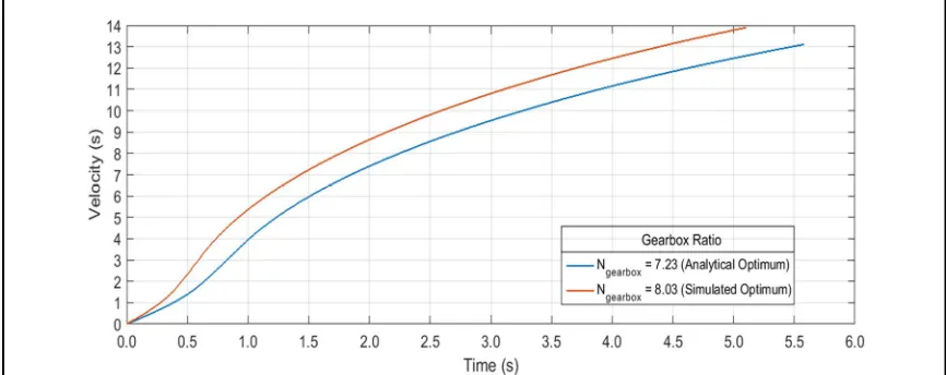
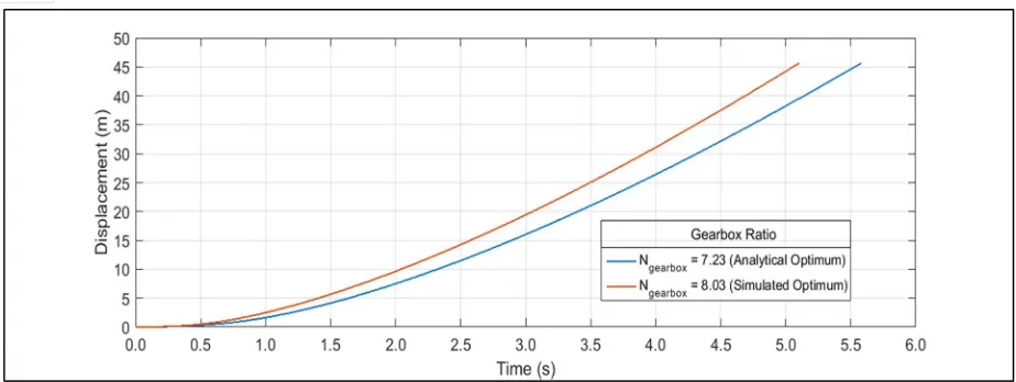
Figure 8: Plot of Displacement versus Time for different gear ratios.

Fig. 7 and 8 illustrate the variation of velocity and displacement with respect to time respectively. It is evident from the graph that although a milder ratio would theoretically achieve a higher top speed for a certain maximum engine rev condition, it takes significantly more time to do so. Hence an aggressive gear ratio proves to be better suited for short sprints and curving tracks, such as those encountered in SAE Baja tracks.

The gearbox ratio has the most significant impact on the top speed of the vehicle and correspondingly on the time and distance required by the vehicle to reach this speed as illustrated by the following table.

Table. I. Variation of vehicle performance parameters with gear ratio.

Gearbox Ratio Top Speed (m/s) Distance covered (m) Time required (s) 150 ft. traversal time

7.23 17.864 161.071 12.851 5.584

8.03 16.084 79.519 7.352 5.107

The table reveals that the vehicle achieves top speed much faster if it were running on the simulated optimum gear ratio. Also, the incurred penalty in terms of maximum achievable speed is reasonably small considering the advantages offered by an aggressive ratio. The time and distance required to achieve top speed is significantly more for the analytical optimum gear ratio as the acceleration of the vehicle approaches zero during the final stages of simulation.

Figure 9: Speed diagram of CVT for different gear ratios.

©IJRASET: All Rights are Reserved

126

As modelling of the wheel slip phase is very crude, the acceleration times predicted by the simulation are not the decisive parameters for gear ratio selection. Also, keeping any gearbox ratio more than that permissible by available traction at the ground results in loss of stability and control of the vehicle. The usefulness of the simulation is in determining the most aggressive ratio beyond which the vehicle starts skidding. This way, the maximum amount of traction is utilized and the best possible acceleration can be obtained. The program accurately considers the loss of torque due to rotational inertia of wheels and transmission components. It also considers the effect of aerodynamic drag on rear axle load. In the vehicle under consideration, the rotational inertia of the wheels is relatively small. This results in only a minor torque loss. Also, the achievable speeds for the vehicle are low, as the engine power is limited to 10 BHP. Owing to these factors, the analytically predicted and simulated optimum ratios are not much far away and their corresponding traversal time for 150 ft. differ by about 8.54%. These results may vary for commercial vehicles.

REFERENCES

[1] Gillespie, T. D. 1996. Fundamentals of Vehicle Dynamics. Warrendale, PA: SAE International. pp. 11-14. 25-27, 97, 111.

[2] Aaen, Olav. 2011. Clutch Tuning Handbook. Racine, WI : AAEN Performance. pp. 8, 9, 14.

[3] Zub, R. W., “A Computer Program (VEHSIM) for Vehicle Fuel Economy and Performance Simulation (Automobiles and Light Trucks). Volume I: Description and Analysis” U.S. Department of Transportation, Research and Special Projects Administration, Transportation Systems Center, Report No. DOT-HS-806-040, October 1981, pp. 2-19 - 2-25.

[4] Rafael Luiz Delmunde et. al., “Analysis of Improvement in Aerodynamics of a Vehicle Type Baja SAE - And the Impact on Performance”, American Journal of Engineering Research, Volume-5, Issue-11, 2006, pp-306-309.

[5] Ricardo Inzunza et. al., “SAE Baja- Drivetrain” Department of Mechanical Engineering, Northern Arizona University, 2014, p. 7.

[6] Prasad Sakat, Adwait Verulkar, Darshan Bamb, Santosh Joshi, “A Case Study on Response of Alloy Gear Steels to Case Carburizingand its Effect on Weight Optimization of a Transmission System”, International Journal of Mechanical and Production Engineering Research and Development, Vol. 7, Issue 2, Apr 2017, 47-56.

[7] Clarence W. De Silva, Martin Schultz, Edward Dolejsi, Kinematic analysis and design of a continuously-variable transmission, Mechanism and Machine Theory, Volume 29, Issue 1, 1994, pp. 149-167.

[8] Christopher Ryan Willis, “A Kinematic Analysis and Design of a Continuously Variable Transmission”, Master Thesis, Department of Mechanical Engineering, Virginia Polytechnic Institute and State University, 19 January 2006, Blacksburg, VA.

[9] Lili Wanga, Dongsheng Lib, Xiaoqiang Lic, Liang Wangd and Weijun Yange, “Coefficient of Friction for Aluminum Alloy Sheet in Contact with Polyurethane Rubber”, Applied Mechanics and Materials, 30 June 2010, Vols. 26-28, pp. 320-325.

[10] B. Bonsen, T.W.G.L. Klaassen, K.G.O. van de Meerakker, M. Steinbuch and P.A. Veenhuizen, “Analysis of Slip in a Continuously Variable Transmission”, Proceedings of IMECE’03 2003 ASME International Mechanical Engineering Congress, Washington, D.C., November 15–21, 2003

[11] Kobayashi, D., Mabuchi, Y., and Katoh, Y., "A Study on the Torque Capacity of a Metal Pushing V-Belt for CVTs," SAE Technical Paper 980822, 1998

[12] Hiroki Asayama, Junji Kawai, Atsushi Tonohata, Masaharu Adachi, "Mechanism of metal pushing belt", JSAE Review, Volume 16, Issue 2, 1995, Pages 137-143.

[13] T. Petry-Johnson, T & Kahraman, A & E. Anderson, N & R. Chase, D. (2008). An Experimental Investigation of Spur Gear Efficiency. Journal of Mechanical Design - J MECH DESIGN. 130. 10.1115/1.2898876.

[14] Yamamoto, T., Matsuda, T., and Okano, N., "Efficiency of Constant Velocity Universal Joints," SAE Technical Paper 930906, 1993.