A Method of Hourly Load Forecasting by Time Series by Recycle of Predicted Values

430

©IJRASET: All Rights are Reserved

A Method of Hourly Load Forecasting by Time Series

by Recycle of Predicted Values

Kuldeep S1, Dr. G S Anitha2

1

Electrical Engineering, Jain University, 2

Dept. of Electrical and Electronics, RV College of Engineering, Vishweshwaraya Technological University

Abstract: Electrical load forecasting is a prime factor in planning of networks, saving costs and balancing supply and demand. As population increases, demand for consumer goods increases, all of which need electricity. While all possible ways are being found to generate electrical power, the ever increasing demand puts a strain on the resources. So a method to predict the load needs to be developed for cost effective supply, for planning networks, planning the generation and distribution. A method of using nonlinear autoregressive neural network model is used to predict the load values as a time series from previous historical load values. Autoregressive neural network time series along with triple exponential smoothing is used and run continuously to further predict from the previously forecasted values.

Keywords: load forecasting, time series, ANN, Holt-Winters, one-lag, multi-lag, bayesian

I. INTRODUCTION

Electric load forecasting is the process of forecasting or predicting loads based on certain parameters. For forecasting, earlier historical data is used as a basis for predicting the next set of values. There are many methods that are used, and being developed for accurate forecasting. There are different classifications of load forecasting based on time, like Very Short Term Load Forecasting, Short Term Load Forecasting, Medium Term Load Forecasting, and Long Term Forecasting. The data required, and the methods used differ with the classification. Also the applications of these methods differ in the way the data is used [1]. This paper deals with Short Term Load Forecasting (STLF). STLF is used to predict load for a time period ranging from hours to a few days. This method is used for scheduling the generation and transmission of power. The data so forecasted helps in decision making regarding supply of power and load distribution and shedding. There are different models and techniques for forecasting. One of the methods which is being constant used and being improved upon is the time series method of forecasting.

II. TIMESERIES

The different methods of load forecasting can be broadly classified into Parametric and Artificial intelligence methods.

Artificial intelligence methods include Fuzzy logic, Expert Systems (ES), Machine Learning, Support Vector Machines (SVM) and Hybrid. Parametric methods require historical data for statistical referencing. The types are parametric method are trending, end use and econometric [2]. Prior series of data varying according to time is necessary for predicting next set of values. Seasonality or variation is captured by Winters method. In a short term, taking per day data, seasonality factor is based on the day. Holt-Winters method allows data to be smoothed over the period of time.

III.HOLT-WINTERSMETHOD

Holt-Winters is a time series method of forecasting. It allows smoothing of time series data. Time series method looks at data as a series of points over a period of time in regularly paced intervals. Holt-Winters model takes into account the three aspects of time series. So this method is also called Triple Exponential Smoothing, as it involves three aspects – the average, slope or trend, seasonality or cyclical repetition over time. These three factors are combined for predicting a value over time [3].

1) Average or Level: Weighted average of the series. Coefficient for level is α.

2) Trend: It is the slope over time, with a value between 0 and 1. Coefficient for trend is β.

3) Seasonality: It is the cyclical repetition of data. A data set that repeats over a period of time is taken as the seasonality. For example, in daily load data of 24 hours, it can be seen that load peaks at certain hours of the day, and is low for some other parts

of the day. Coefficient for seasonality is γ.

Two methods that Holt-Winters model can be used are additive and multiplicative [4].

431

©IJRASET: All Rights are Reserved

IV.METHODOLOGY

In this paper, loads for a particular area in Bengaluru city are taken as a data set for prediction using nonlinear autoregressive neural network (NARNET) for time series prediction and Holt-Winters method for triple exponential smoothing.

Sample data is taken from Bengaluru Electric Supply Company (BESCOM) in the month of April 2019, for the area HSR layout, with residential and commercial establishments like hotels and shops in almost equal measure [5]. One day data for 23 hours is used for training the network. After subsequent training till error is reduced, the trained network is applied on a new set of data for forecasting.

The data to be trained and predicted are both normalized first. This is done by dividing all values by the largest value in the set. In this way, the data is reduced to values between 0 and 1. Later, the forecasted values are denormalized to get the actual numbers.

V. FLOWCHARTOFTHEMETHOD

One lag prediction model is used to obtain one variable delay. There are two types of time series predictions, one lag and multi-lag. In one lag prediction, if there are 5 variables, v1, v2, v3, v4, v5, the network is run with a lag, or delay by one variable, from v2 to v5, to predict the sixth variable v6.

The method proposed here is continuous recycling of variables for forecasting the next set of variables, or load. Each time the network is run, it predicts the next hour load. This value will be a part of the data set to predict the next hour load, and so on. The forecasted data is compared with actual data.

432

©IJRASET: All Rights are Reserved

VI.LOADVARIATIONS

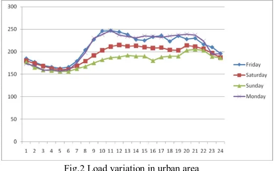
A sample set of loads is taken here for HSR layout area of Bengaluru city. A comparison between load on weekends and weekdays can be made here.

Fig.2 Load variation in urban area

The graph shows that loads are more on weekdays, as the Friday and Monday graphs nearly coincide with each other. The load starts increasing from about 7 am, peaks between 9 am and 1 pm. The afternoon loads are almost constant. The load variation graph depends on the type of area considered. HSR Layout is an area with residential and commercial establishments. This type of graph may not be the same in an area with only residences, or more of industrial and heavy machinery usage.

VII. RESULTS

The NARNET time series is trained using Bayesian regularization backpropagation, which varies weights and biases according to Levenberg-Marquardt optimization [5]. The network has one input layer, one hidden layer with 40 neurons.

Data considered is for two days, April 4th and 5th of 2019 for HSR Layout. 23 hour data from April 4 is considered for training the network.

The methodology followed in this paper is the network is repeatedly trained to get minimum error, with loads of April 4th. The trained network is then applied to get the 24th hour value as a forecast. This data becomes an input for the next set of data for prediction, which will be the next day, April 5th. Likewise, as per the one lag method of time series prediction, the data keeps getting circulated one step at a time till a completely new set of data for the next day (Apr 5th) is forecasted. Holt-Winters multiplicative method is applied for smoothing.

The study below gives a comparison of results based on the number of epochs and the accuracy.

Fig. 3 Epochs 1570

Regression is 0.94, SSE is 0.79, MSE is 0.03.

433

©IJRASET: All Rights are Reserved

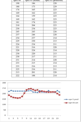
Table I. Predicted values in 2000 epochs April 04 April 05 (actual) April 05 (predicted)

190 186 220

180 173 229

174 165 223

169 162 223

164 159 223

169 162 223

181 174 223

210 204 223

230 234 223

245 243 226

237 246 228

234 237 214

229 230 213

224 234 211

221 216 228

220 224 214

230 220 213

230 217 211

231 214 228

233 215 214

233 216 213

225 216 211

213 201 228

222 188 214

Fig.4 Epochs 2000

Regression is 0.97, SSE is 0.51, MSE is 0.02

A. Equations

The simplified calculation for Holt-Winters method is listed below [6]:

1) Season (forecast_data x 24)/sum_forecasted Since the data is taken on a day basis with 24 hours, the coefficient is 24.

2) Level is average of series, given by ratio of each value to season.

3) For trend, the coefficient is assumed to be 0.05.

SSE is Sum of Squared Errors. It is given by the sum of the differences between actual value and forecasted value.

434

©IJRASET: All Rights are Reserved

VIII. CONCLUSIONS

Further testing with different data and epochs give a relationship between the number of epochs and accuracy. As can be seen from the graphs and their respective error values, higher the number of times the time series is run, better the results. Here, the number of epochs is set at maximum of 2000, as the results deteriorate above this number.

REFERENCES

[1] Y.W. Lee1, K.G. Tay, Y.Y. Choy, Forecasting Electricity Consumption Using Time Series Model, International Journal of Engineering & Technology, 7 (4.30) (2018) pp 218-223

[2] Emiyamrew Minaye, Melaku Matewose, Long Term Load Forecasting of Jimma Town for Sustainable Energy Supply, International Journal of Science and Research (IJSR), Volume 5 Issue 2, February 2016, ISSN (Online): 2319-7064, pp 1500-1504

[3] Sergi Cunill Cols, Load forecasting Using Holt-Winters Method, Universitat Politecnica de Catalunya

[4] Maya Shelke1, Prashant Dattatraya Thakare, Short Term Load Forecasting by Using Data Mining Techniques, International Journal of Science and Research (IJSR), Volume 3 Issue 9, September 2014, ISSN (Online): 2319-7064

[5] https://bescom.org/daily-statistics-of-operations-wing-april-2019/