Non-Linear Dynamics (Vibration Analysis) of a Flexible
Single Link Cartesian Manipulator
G. Laxmareddy
1, G. Satish babu
21Student, 2Professor, Department of Mechanical Engineering, JNTUH College of Engineering, Kukatpally, Hyderabad, India,
Abstract: The present work deals with the non-linear vibration analysis of a harmonically excited single link roller-supported flexible Cartesian manipulator with a mass at the end. The governing equation of motion of this system is developed using D’ Alemberts principle. Using generalized Galerkin’s method the governing equation of motion is reduced to the second-order temporal differential equation of motion. In order to study the stability and bifurcations of the system the nonlinear equation of motion is solved using method of multiple scales. The influence of amplitude of the base excitation and mass ratio on the steady state response of the system is investigated for simple resonance conditions. Critical bifurcation points are determined from the fixed-point responses and periodic responses are found for different system parameters. The perturbation analysis results are compared with the previously published experimental work and are found to be in good agreement. This work will be useful for designing of a flexible manipulator.
I. INTRODUCTION
control of a flexible-link manipulator. The problem of modelling and controlling the tip position of a one-link flexible manipulator is considered. The proposed model has been used to investigate the effect of the open-loop control torque profile, and the payload. Barun Pratiher, Suman Bhowmick [9] Presented work on Nonlinear dynamic analysis of a Cartesian manipulator carrying an end effector placed at an intermediate position. Nonlinear dynamic analysis of a Cartesian manipulator carrying an end effector which is placed at different intermediate positions on the span is theoretically investigated with a single mode approach.
II. MATHEMATICAL MODELING
[image:2.595.220.384.283.357.2]A. Derivation Of The Temporal Equation Of Motion
Fig. 1 shows a single link flexible Cartesian manipulator with mass M at the free end and roller supported at the other end which is subjected to harmonic excitation. The roller-supported end is assumed to have periodic motionY tb( )Zcos1t where Z and are amplitude and
1
frequency of the base excitation. The motion is considered to be in the x-y plane. Here, the manipulator is modeled as an Euler–Bernoulli beam with a tip mass.
Using D’ Alembert’s principle the governing differential equation of motion of the system is derived as:
2 3
2 0
2 2
0 0
2 1
3 2
( ) ( )
( ) ( )
( )
1 1
2
ssss s ssss s ss sss ss s
s b s ss
L
s ss b d
s
L s
ss s
s
E I v v v v v v v
A v v v v d M v Y v v
v v A Y L s A v C v d
v A v v v d d M v v v d
v
A v( Yb) C vd
( ( )P t vs)s 0
(1)
Here V denotes the transverse displacement in y direction. (·) and ( s) denote, respectively, the first derivative with respect to time t and displacement along the elastic line s. Here, E, I,
, A,L, and m are the Young modulus, moment of inertia, mass density, cross-sectional area, length of the cantilever beam, and mass of the beam (i.e.
AL), respectively. c is the viscous damping constant. To discretize the governing equation of motion (1) one may use the following assumed mode expression:V (s, t) = rvy(s)u(t). (2)
Here, r is the scaling factor u(t) is the time modulation and Vy (s) is the eigenfunction of the cantilever beam with tip mass, which is given by
sin sinh
( ) co s co sh sin sin h
cos cosh
l l
s s s s s
l l
One may determine L from the following equation:
1 c o s Lc os h L M L c os Lsin h L s in Lco sh L 0
A L
The following non-dimensional parameters are used in the
analysis: 1 2
1 2
, s, , ,
s s
s r
x t r
L L
0 1
0 1 4
, , , ,
c c
P P
M EI Z
m P P k
AL P P AL r
3 2 2 2 2
1 2 3 4 1 1
2
5 1 1 6 2
2
( cos( )
cos( ) cos( ) ) 0
q q q
q q q q q q
q
(3)
The solution of the above equation is carried out using perturbation method as described in the following section.
B. Perturbation Analysis
As the equation of motion (3) contains many non-linear terms, it is very difficult to find the close form solution. Therefore, one may go for the approximate solution of Eq. (3) by using perturbation techniques. Here, method of multiple scales is used to find the approximate solution. In this method the displacement u can be represented in terms of different times scales (T0, T1) and a book keeping parameter
as follows:
20 0 1 1 0 1
, , ,
q q T T q T T O
(4)
where T0=
, T1=
, and the transformation of first and second time derivatives are given by
20 1
d
D D O
d
2
2 2
0 0 1
2 2
d
D D D O
d (5)
Here, D0 = partial differentiation w.r.tT0 and D1 = partial differentiation w.r.t T1. Substituting Eqs. (4) and (5) into Eq. (3) and equating coefficients of like powers of yields the following expressions:
2
0 0 0 0
D q q (6)
2 3 2 2
0 1 1 0 1 0 0 0 1 0 2 0 0 0
2 2 2 2
3 0 0 0 4 0 5
2 2
c o s ( ) c o s ( )
D q q D D q D q q q D q
D q q q
(7)
General solution of Eq. (6) can be written asq0A T( ) exp(1 iT0)A T( ) exp(1 iT0)
Substituting Eq. (6) into Eq. (7) leads to
2 2 2
0 1 1 (2 1 2 3 1 3 2
D q q iD A i A A A A A
2 3
3 0 1 2 3 0
2 2 2 2
4 0 4 0
2
4 5 0
)exp( ) exp(3 )
1 1
exp (2 ) exp ( 2)
2 2
1
exp ( ) 2
A A iT A iT
A i T A i T
AA i T cc
(8)
Where: cc – complex conjugate of preceding terms. Though the actual response of the system is bounded, due to the presence of secular or small divisor terms in equation 8, the solution of the system sometimes will not be bounded. For a bounded solution, these terms should be removed. Equation 8 contains secular or a small divisor terms when frequency of excitation is nearly equals to 1or three times the natural frequency. In simple resonance case both forcing and nonlinear parametric excitation terms will contribute to the resonance condition. In sub-harmonic resonance condition only nonlinear parametric term contribution is felt.
C. Simple Resonance case 1
:
In the case of simple resonance, one may use the detuning parameter to express the nearness of to 1 as
1 ,
O(1) (9)
In order to eliminate the secular or small divisor terms substitute 9 into 8 we obtain the following equation.
2 2 2 2 2
1 2 3 4 1
1
2 2 3 3 exp ( )
2
iA i A A A A A A A A iT 2 4 5 1
1
exp ( ) 0 2
AA i T
(10)
Substituting A in the polar form i.e.
1
( ) 1
1 ( ) 2
i T
A a T e
and separating the real and imaginary parts yields the following expressions:
2 4 2 5
1 sin 8 2
a a a
Here,
' 1
T
, and T1. For steady state response
a0,0
, 'a and ' are equal to zero. Eliminating
from equations 11 and 12 one may find a fifth order polynomial in2
a
, which can be expressed as :10 8 6 4 2
5 4 3 2 1 0 0
Q a Q a Q a Q a Q a Q (13)
Where:
8 4
0 5
1 16
Q
2 4 2 4 2 2 8 3
1 5 5 4 5
1 1 1
4 4 8
Q
2 4 4 2 4 3 2 8 2 2
2 4 5 4 5 1 2 5 4 5
3 1 3 11
8 8 16 3 32
Q
2
2 4 2 4 2 4 3 2 4 3 8 3
3 4 4 1 2 5 1 2 4 5 4 5
9 1 9 3 1
65 64 256 3 32 3 128
Q
2
4 3 4 3 2 8 4
4 1 2 4 5 1 2 4 4
9 3 9
512 3 256 3 4096
Q
, and
2 4 3 2
5 1 2 4
9
4096 3
Q
Equation 13 is an implicit equation for amplitude of the response as a function of the external detuning parameter
, tip mass M and the amplitude of the base excitation Z. Equation 13 does not have trivial state response, therefore the response is found by numerically solving it or numerically solving the reduced equations 11 and 12 simultaneously. Newton’s method is used to solve numerically the polynomial equation to find the response of the system. The response can be found by numerically solving temporal equation 3 by using runge-kutta fourth order method.From equation 3.16, the first order nontrivial steady state approximate solution can be given by.cos( ) ( )
qa O (14)
III. NUMERICAL RESULTS AND DISCUSSIONS
Metallic beam with the following parameters is considered from the Cuvalci (2000).
Length (L) 0.336 m Cross-section area (A) 40.464 x 10⁻⁶ m2
Moment of inertia (I) 8.669867 x 10⁻¹² m4
Young’s modulus (E) 1.5848 x 10¹¹ N/m2
Damping constant (Cd) 0.11 N-s/m Mass density (
) 7830 kg/m3
Scaling parameter (
r
) 0.1 Book-keeping parameter(
) 0.1The nonlinear response for this system is determined for different values of amplitude of harmonic support motion
( )
Z
and payload mass M for the simple resonance condition.A. Simple Resonance Condition
1
The resonance condition takes place when the frequency of the support motion of the
1 nearly equals to the fundamental frequency of the system. Figure 3.2 shows the frequency response curves for simple resonance case for the non-dimensionalFig.3.1. Frequency response for simple resonance case for mass ration of 1.8787 and base excitation of 0.00372.
[image:5.595.210.375.110.206.2]It is observed from the frequency response curve that the system does not possess any trivial state response. So, one may note that manipulator will always oscillate about its equilibrium position with an amplitude equal to the nontrivial response as shown in fig.3.1. When the manipulator is started, with increase in frequency of external excitation, the response amplitude of the manipulator increases and it will reach a critical value, which is saddle node bifurcation point. At this point further increase in frequency, the system will experience a jump up phenomenon (observed in blue line of fig.3.3), which leads to sudden increase of amplitude. The
system may fail due to this sudden jump. It is shown in figure 3.1 that the system experiences an upward jump at frequency
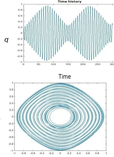
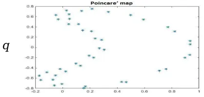
equal to 0.93 with a jump length equals to 0.3.The fundamental frequency of the system is 3.49 Hz therefore the system resonates at frequency equal to 3.24 Hz. When excitation frequency is swept down with decrease in frequency the response amplitude increases. This situation may occur when prime mover of the manipulator is stopped and in that case the system will experience a jump down phenomenon, which leads to catastrophic failure. It is observed that the system has a bi-stable region before the saddle-node bifurcation point. The initial condition will play a very important role to determine the actual system response.Figure 3.2. shows the time response, phase portrait, and Poincare’s section at the critical point. The time response is obtained by solving the temporal equation of motion using fourth order Ringe-Kutta method. While transient response of the system with initial point (a=0.326, gamma=0.1)give a beating type phenomenon, the steady state response of the system is periodic. The phase portrait and Poincare’s section for transient and steady state response are shown below.
a
Time
[image:5.595.191.391.433.707.2]Fig. 3.2. Time response, phase portrait, and Poincare’s section at the critical point respectively.
[image:6.595.195.386.365.428.2]Figures below show the variation of the response of the system with varying mass ration or excitation amplitude of base.
Fig 3.3 Frequency response curve for simple resonance case for mass ration of 1.8787 and excitation amplitude is z bar= 0.05, 0.0125 respectively.
Fig 3.4 Frequency response curve for simple resonance case for excitation amplitude of 0.02 and mass ratio = 0.5656, 4.6968 respectively.
From figure 3.3 we can see that the jump length and maximum response will decrease with decrease in the excitation amplitude. The variation of response is marginal with the variation of excitation amplitude. With decrease of excitation amplitude the saddle point shifts towards the fundamental frequency.
From figure 3.4 the bifurcation point shifts towards left side with increase of mass ratio i.e. the system fails at lower frequency for a system with higher mass ratio. The maximum amplitude and jump length decreases with increase in the mass ratio value.
IV. CONCLUSION
Non-linear response of a flexible single link roller-supported Cartesian manipulator with payload subjected to a harmonic base excitation is investigated using the method of multiple scales. Frequency responses are plotted and their stability and bifurcations are studied for different values of mass ratio and amplitude of base excitation for simple resonance condition. In simple resonance case, the system does not possess any trivial state response. In this case, with decrease in amplitude of external excitation, the maximum value of nontrivial response amplitude remained almost same and system undergoes a catastrophic failure due to jump up phenomena at saddle-node bifurcation point. The designer of the manipulator may use the simplified polynomial equation 13 to find the response amplitude to successfully design a new similar manipulator without having vibration problem when the system is operating near the simple resonance frequency. The present work can be extended to sub-harmonic resonance condition.
A. Appendix
The system fundamental frequency
1 4 2 s
h h
2
19 18 20
1 2
2 2 2
3 s
h h h
r
h h h
q
q
2
5 6 8 7
1 4
2
2 2 2 2 2 2 2
h h h h
h h
r
m m
h h h h h h
2 13 11 12 3
2 2 2
h
h h
r
m
h h h
15 16 17 1
4
2 2 2 2
, 5 2
h h h h
Zr k
m
h h h h
2 d s C A
Here the expressions for h1, h2, . . . , h20 are given below:
1 1
0
( ) ,
h
x dx
1 2
2 0
( ) ,
h
x dx 1
2 3
0 0
,
x d
d x
h d x dx
dx d
2 1 1 4 2 0 , xd x d x
h d d x dx
dx dx
2 1 2 5 2 0 ,d x d x
h x dx
dx dx
2 2 1 1 6 2 0 0 , x d d xh d d x dx
dx d
2 2 1 7 2 0 0 , x d d xh d x dx
dx d
2 1 2 8 0 ( ) , d xh x dx
dx
h9h h4, 10h h8, 11h h3, 12h h6, 13h7,1 4 14 4 0 ( ) ( ) , d x
h x dx
dx 2 1 15 2 0
1 d x d x ( ) ,
h x x dx
dx dx
2
1
16 2
0
( ) ,
d x d x
h x dx
dx dx
2 1
17 0
( ) ,
d x
h x dx
dx
21 4
18 4
0
( ) ( ) ,
d x d x
h x dx
dx dx
2 1 19 2 0 ( ) , d xh x dx
dx
2 3
1
20 2 3
0
( ) ,
d x d x d x
h x dx
dx dx dx
21 19.
h h
REFERENCES
[1] C. W. S. TO, Vibration of a cantilever beam with base excitation and tip mass, Dept. of ME, University of Calgary, 1981.
[2] Olkan Cuvalci, The effect of Detuning parameters on the absorption region for a coupled system: A numerical and experimental study, Journal of sound and vibration (2000) 229(4), 837-857.
[3] Lawrence D. Zavodney, A Theoretical and experimental investigation of parametrically excited nonlinear mechanical systems, Virginia Polytechnic Institute and State University, Dec 1987.
[4] Rajesh Kumar Moolam, Dynamic modeling and control of flexible manipulators, Politecnico di Milano, Dept. of ME, 2013 – XXVI.
[5] Jinyong Ju, Wei Li, Mengbao Fan, Yuqiao Wang, and Xuefeng Yang, Nonlinear modelling and dynamic stability analysis of a flexible Cartesian robotic manipulator with base disturbance and terminal load, Mech. Sci., 8, 221–234, 2017.
[6] R. C. Kar and T. Sujata, Parametric instability of an elastically restrained cantilever beam, Computers and structures Vol.34, No.3, pp.469-475, 1990. [7] Atef A. Ataa, Waleed F. Faresb, Mohamed Y. Sa'adehc, “Dynamic analysis of a two-link flexible manipulator subject to different sets of conditions”, Procedia
Engineering 41 ( 2012 ) 1253 – 1260.
[8] Carmelo di, Castri and Arcangelo Messina, “Vibration analysis of Multilink Manipulators Based on Timoshenko Beam theory”, Volume 2011,Article ID 890258.
[9] Barun Pratiher, Suman Bhowmick, “Nonlinear dynamic analysis of a Cartesian manipulator carrying an end effector placed at an intermediate position”, Nonlinear Dyn (2012) 69:539–553.