Abstract— In this paper a human lower limb cinematic
analysis is realized, by using a computerized method with a flexible character, easy to implement onto computer. Through this method we obtain the generalized coordinates motion laws of the knee cinematic joint from the equivalent model of the human lower limb. These laws are useful for a new human knee prosthesis design.
Index Terms—cinematic, knee prosthesis, human lower
limb.
I. INTRODUCTION
ANY researchers have been developed different methods for study the human lower limb cinematic [1], [2], [3], [4].
The cinematic methods aim is to study different motion types of the human lower limb in order to improve the athletes’ performances or to design new human lower limb prosthesis.
The cinematic analysis of a mechanical model consists in solving two important problems: cinematic direct problem and cinematic inverse problem.
In the cinematic direct problem’s frame, the displacements from cinematic joint are known, and it will be determined the positions – orientation, speeds and accelerations of the mechanism elements or some characteristic points onto the analyzed mechanism.
In the cinematic inverse problem, the cinematic parameters for some characteristic points motion are known, and it will be determined the cinematic parameters of the cinematic joints relative motions.
With these, in the cinematic analysis context, we identify many problems such as:
- Positional problem; - Speed problem; - Accelerations problem.
Each of these problems presents a direct or inverse aspect.
Manuscript received March 29, 2011; revised March 29, 2011. This work was supported in part bythe Roumanian. Department of Research under Grant CNCSIS PNII – RU – PD – 2009 – 1 code: 55/28.07.2010.
C. Copilusi is with the Faculty of Mechanics, University of Craiova. Calea Bucuresti no. 113. Romania (corresponding author to provide phone: +04 0747222771; e-mail: [email protected]).
M. Marin, is with the Faculty of Mechanics, University of Craiova. Calea Bucuresti no. 113. Romania (e-mail: [email protected]).
L. Rusu is with the Faculty of Educational Physics and Sport. University of Craiova. Brestei street. Romania (e-mail: [email protected]).
II. HUMANLOWERLIMBCINEMATICANALYSIS The method used in this paper has a flexible character and assures an interface for dynamic analysis especially for finite element modeling of spatial and planar mobile mechanical systems [5].
For the cinematic analysis the cinematic model presented in figure 1, will be considered. The cinematic model analysis will be performed only for walking activity, for a single gait. The cinematic parameters variation laws were obtained by processing with the MAPLE software aid the mathematical models which are defining the human lower limb experimentally cinematic analysis.
From a structural viewpoint, the cinematic chain it consists in 8 rotation joints.
The
r
i position vectors in theT
i1 reference coordinate system are:A New Knee Prosthesis Design Based on
Human Lower Limb Cinematic Analysis
Cristian Copilusi, Mihnea Marin and Ligia Rusu
[image:1.595.323.525.393.756.2]M
0, ,0
.; 0 , , 0 ; 0 , , 0
; 0 , , 0 ; , 0 , 0
; 0 , , 0 ; 0 , , 0
; , 0 , 0 ; 0 , , 0
8 8 8
7 7 8
6 6 7
5 5 6
4 4 5
3 3 4
1 1 2
2 2 3
1
T
T T
T T
T T
T T
cx cx
L S
L r
L r
L r
L r
L r
L r
L r
L r
(1)
The connectivity order will be:Cx - 1 - 2 - 3 - 4 - 5 - 6 - 7 - 8
A. Position calculus The position vectors are:
cx Tz y x
W
r
r
r
r
r
1
1,
1,
1
1
(2)
2 2 2
2
1 2r
,
r
,
r
r
W
r
x y z
T
(3)
3 3 3
3
23
r
,
r
,
r
r
W
r
x y z
T
(4)
4 4 4
4
34
r
,
r
,
r
r
W
r
x y z
T
(5)
5 5 5
5
4 5r
,
r
,
r
r
W
r
x y z
T
(6)
6 6 6
6
56
r
,
r
,
r
r
W
r
x y z
T
(7)
7 7 7
7
87
r
,
r
,
r
r
W
r
x y z
T
(8)
8 8 8
8
78
r
,
r
,
r
r
W
r
x y z
T
(9)
8 8 8
8
88
S
,
S
,
S
S
W
S
x y z
T
(10)Where:
0, ,0
.; 0 , , 0 ;
0 , , 0
; 0 , , 0 ;
, 0 , 0
; 0 , , 0 ;
, 0 , 0
; 0 , , 0 ;
0 , , 0
8 8 8
7 7 8
6 6 7
5 5 6
4 4 5
3 3 4
2 2 3
1 1 2
1
L S
L r
L r
L r
L r
L r
L r
L r
L r
T
T T
T T
T T
T cx cx T
(11)
The
r
MCx vector, has the following expression:8 8 7 6 5 4 3 2
1
r
r
r
r
r
r
r
S
r
r
MCx
(12)Changing the versors base at crossing from a reference coordinate system to another (introducing the coordinate transformation matrices):
W1
ACx1
WCx (13)
W
2
A
12
W
1
A
Cx2
W
Cx (14)
W3
A23
W2
ACx3
WCx (15)
W4
A34
W3
ACx4
WCx (16)
W5
A45
W4
ACx5
WCx (17)
W6
A56
W5
ACx6
WCx (18)
W7
A67
W6
ACx7
WCx (19)
W
8
A
78
W
7
A
Cx8
W
Cx (20)By analyzing the (13) ... (20) relations we observe that:
A
Cx2
A
12
A
Cx1 (21)
A
Cx3
A
23
A
12
A
Cx1 (22)
ACx4
A34 A23 A12 ACx1 A34 ACx3
(23)
45 4
1 12 23 34 45 5
Cx
Cx Cx
A
A
A
A
A
A
A
A
(24)
56 51 12 23 34 45 56 6
Cx
Cx Cx
A A
A A A A A A A
(25)
12 1 67 6
23 34 45 56 67 7
Cx Cx
Cx
A
A
A
A
A
A
A
A
A
A
(26)
23 12 1 78 7
34 45 56 67 78 8
Cx Cx
Cx
A
A
A
A
A
A
A
A
A
A
A
(27)
Based on (21)... (27) relations we identify the coordinates transformation matrices for each cinematic joints, with
90 1 ,i
i
, and
i
1
,
8
.
Point: A, B, C, D, E, F, G, H and M positions in rapport
with
T
cx coordinate system, bounded to the coxae bone, will be identified through relations:
CxT T
A r W
r CX
1 (28)
Cx
CxT Cx T T
B r W r A W
r CX 1 2 1 (29)
Cx
Cx TCx Cx T Cx T T
C
W A A r
W A r W r r CX
1 12 3
1 2
1 (30)
Cx
Cx TCx Cx
T
Cx Cx
T Cx
T T
D
W A A A r
W A A r
W A r W
r r CX
1 12 23 4
1 12 3
1 2
1
(31)
Cx
CxT Cx
Cx
T Cx
Cx T
Cx Cx
T Cx
T T
E
W A A A A r W A
A A r W A A r
W A r W r r CX
1 12 23 34 5
1
12 23 4
1 12 3
1 2
1
(32)
Cx
Cx TCx Cx T
Cx Cx
T Cx Cx T
Cx Cx T Cx T T
F
W
A
A
A
A
A
r
W
A
A
A
A
r
W
A
A
A
r
W
A
A
r
W
A
r
W
r
r
CX
1 12 23 34 45 6
1 12 23 34 5 1
12 23 4 1
12 3
1 2
1
Cx
Cx T Cx Cx T Cx Cx T Cx Cx T Cx Cx T Cx Cx T Cx T T G W A A A A A A r W A A A A A r W A A A A r W A A A r W A A r W A r W r r CX 1 12 23 34 45 56 7 1 12 23 34 45 6 1 12 23 34 5 1 12 23 4 1 12 3 1 2 1 (34)
Cx
Cx T Cx Cx T Cx Cx T Cx Cx T Cx Cx T Cx Cx T Cx Cx T Cx T T H W A A A A A A A r W A A A A A A r W A A A A A r W A A A A r W A A A r W A A r W A r W r r CX 1 12 23 34 45 56 67 8 1 12 23 34 45 56 7 1 12 23 34 45 6 1 12 23 34 5 1 12 23 4 1 12 3 1 2 1 (35)
Cx
CxT Cx Cx T Cx Cx T Cx Cx T Cx Cx T Cx Cx T Cx Cx T Cx Cx T Cx T T M
W
A
A
A
A
A
A
A
A
S
W
A
A
A
A
A
A
A
r
W
A
A
A
A
A
A
r
W
A
A
A
A
A
r
W
A
A
A
A
r
W
A
A
A
r
W
A
A
r
W
A
r
W
r
r
CX
1 12 23 34 45 56 67 78 8 1 12 23 34 45 56 67 8 1 12 23 34 45 56 7 1 12 23 34 45 6 1 12 23 34 5 1 12 23 4 1 12 3 1 2 1 (36)B. Speed calculus
We follow to determine the M point speed in rapport with
cx
T
reference system. For this we differentiate successively the (28) ... (36) relations, but for achieve this calculus is necessary to build the anti symmetric matrices for each joint, like this form: 0 0 0 ~ Cxj Cxj Cxi Cxi Cxi Cxi Cxi
, withi
,
j
1
,
8
(37)For this:
1 ~ 11 Cx Cx
Cx
A
A
(38)
3 ~ 12 2 Cx CxA
A
(39)
3 ~ 23 3 Cx CxA
A
(40)
4 ~ 34 4 Cx CxA
A
(41)
5 ~ 45 5 Cx CxA
A
(42)
7 ~ 56 6 Cx CxA
A
(43)
7 ~ 67 7 Cx CxA
A
(44)
8 ~ 78 8 Cx CxA
A
(45)For each: A, B, C, D, E, F, G, H and M point we obtain:
Tcx
0
Av
(46)
Cx
Cx
Cx TTcx
B
r
A
W
v
1
1
~
2
0
(47)
Cx
CxT Cx Cx Cx T Tcx C
W
A
r
W
A
r
v
2 12 ~ 3 1 1 ~ 20
(48)
Cx
CxT Cx Cx T Cx Cx Cx T Tcx D W A r W A r W A r v 3 23 ~ 4 2 12 ~ 3 1 1 ~ 2 0
(49)
Cx
CxT Cx Cx T Cx Cx T Cx Cx Cx T Tcx E W A r W A r W A r W A r v 4 34 ~ 5 3 23 ~ 4 2 12 ~ 3 1 1 ~ 2 0
(50)
Cx
CxT Cx Cx T Cx Cx T Cx Cx T Cx Cx Cx T Tcx F W A r W A r W A r W A r W A r v 5 45 ~ 6 4 34 ~ 5 3 23 ~ 4 2 12 ~ 3 1 1 ~ 2 0
(51)
Cx
Cx T Cx Cx T Cx Cx T Cx Cx T Cx Cx T Cx Cx T Cx Cx Cx T Tcx HW
A
r
W
A
r
W
A
r
W
A
r
W
A
r
W
A
r
W
A
r
v
7 67 ~ 8 6 56 ~ 7 5 45 ~ 6 4 34 ~ 5 3 23 ~ 4 2 12 ~ 3 1 1 ~ 20
(53)
Cx
CxT Cx Cx T Cx Cx T Cx Cx T Cx Cx T Cx Cx T Cx Cx T Cx Cx Cx T Tcx M W A S W A r W A r W A r W A r W A r W A r W A r v 8 78 ~ 8 7 67 ~ 8 6 56 ~ 7 5 45 ~ 6 4 34 ~ 5 3 23 ~ 4 2 12 ~ 3 1 1 ~ 2 0
(54)C. Acceleration calculus
These will be obtained by differentiating successively the (46) ... (54). For A, and B, we will obtain the accelerations
from (55) and (56) relations. Similarly, we obtain the accelerations of the following points: C, D, E, F, G, H. The
acceleration for M point is given by (57) relation.
Tcx
0
A
a
(55)
T Cx Cx
Cx
CxCx Cx Cx T Tcx B W A r W A r a 1 1 ~ 1 ~ 2 1 1 ~ 2 0
(56)
Cx Cx T Cx Cx T Cx Cx Cx Cx T Cx Cx Cx T Tcx M W A r W A r W A r W A r a 2 12 ~ 12 ~ 3 2 12 ~ 3 1 1 ~ 1 ~ 2 1 1 ~ 2 0 (57)
T
Cx
Cx Cx Cx T Cx Cx T Cx Cx T Cx Cx T Cx Cx T Cx Cx T Cx Cx T Cx Cx T Cx Cx T Cx Cx T Cx Cx T W A S W A S W A r W A r W A r W A r W A r W A r W A r W A r W A r W A r 8 78 ~ 78 ~ 8 8 78 ~ 8 7 67 ~ 67 ~ 8 7 67 ~ 8 6 56 ~ 56 ~ 7 6 56 ~ 7 5 45 ~ 45 ~ 6 5 45 ~ 6 4 34 ~ 34 ~ 5 4 34 ~ 5 3 23 ~ 23 ~ 4 3 23 ~ 4 III. NUMERICAL PROCESSING
For the cinematic analysis we consider known the geometrical elements. The calculus algorithm was elaborated with the MAPLE software’s aid. The geometrical elements dimensions are: Lcx=15,744 mm; L1=12,5 mm; L2=12,5mm; L3=385 mm; L4=5 mm; L5=325 mm; L6=10,7 mm; L7=61,85 mm; L8=50,42 mm.
The generalized coordinate system variations from the 8 joints equivalent to the human lower limb are presented in the cinematic diagrams (figures: 2, 3, 4, and 5).
In figure 6, the human locomotion system’s 3D virtual model is presented. This was designed by and simulated with the MSC NASTRAN software’s aid. For virtual simulation we follow the procedures from [6] and we implement the motion laws resulted from the analysis developed previously (figures 2 3, 4 and 5), on a human subject without locomotion disabilities.
IV. CINEMATIC RESULTS APPLICATION ONTO KNEE PROSTHESIS MECHANICAL SYSTEMS
Based on cinematic motion laws imposed for a knee prosthesis mechanism, we design a 3D virtual model of cam mechanism prosthesis, with the CATIA V5 R16 aid. This mechanism is similar with a one designed for human ankle prosthesis [7].
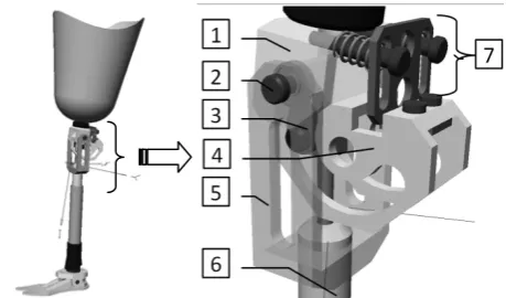
We integrated the FESTO YSR-20-25-C shock absorber in the prosthesis resistance structure, which enables some axial adjustments with a view to establishing the prosthesis alignment. Figure 7 shows the new knee prosthesis design. This is where we identify 1-femur component, 2-cilindrical joint, 3- cam follower, 4- cam, 5- tibia component, 6-FESTO shock absorber, 7-aditional shock absorber mechanism. After simulating the virtual model and validating the cam mechanism through calculation, we executed and adapted this prosthesis in accordance with an amputee's needs and suggestions. In figure 8, we present an aspect from the new prosthesis experimental tests, which were performed with SIMI Motion’s aid.
Fig. 2. q3 variation angle [degrees], corresponding with the equivalent hip joint
[image:5.595.324.547.47.265.2]Fig. 3. q5 variation angle [degrees], corresponding with the equivalent knee joint
Fig. 4. q7 variation angle [degrees], corresponding with the equivalent ankle joint
Fig 5. q8 variation angle [degrees], corresponding with the equivalent foot joint
[image:5.595.63.270.48.243.2] [image:5.595.68.271.288.483.2] [image:5.595.312.549.301.503.2] [image:5.595.64.279.523.732.2]
Fig. 7. Virtual model of the prosthesis used in human knee disarticulations
V. CONCLUSION
For cinematic modeling we use a method which is based on simple matrices formalism with the possibility to implement on a computer program for the direct or inverse cinematic analysis. This method is valid for planar and spatial cinematic mechanisms with possibility to study the cinematic parameters in the absolute or relative motion mode. For the mathematical models processing corresponding to the cinematic analysis, a program under MAPLE programming language was elaborated.
It was elaborated a cinematic scheme for the human lower limb equivalent mechanism, based on some specialty literature references, but also with proper observations mainly for knee joint. Mathematical model were elaborated for position, speeds and accelerations determination, for some interest points, used for experimental modeling, according with a new prosthesis design for knee joint.
The novelty element which assures the prosthesis models design is represented by cam mechanisms.
Based on an experimental cinematic analysis of these prostheses, by using SIMI Motion software, the angular amplitude developed by this mechanism is appropriate with the one developed by a healthy human subject. So, for the human knee joint replacement mechanism, the angular amplitude for walking activity was 63 degrees (figure 9), and the one developed by a healthy subject was 65 degrees [9], [10].
The prosthesis presented in this paper is cheap, in comparison with the ones manufactured by the specialized
prosthetic centers. The knee mechanism functionality validates the cinematic analysis of the human lower limb.
ACKNOWLEDGMENT
The research work reported here was made possible by Grant CNCSIS –UEFISCSU, project number PNII – RU – PD – 2009 – 1 code: 55/28.07.2010.
REFERENCES
[1] R. M. Kiss, L. Kocsis, and Z. Knoll. Joint kinematics and spatial temporal parameters of gait measured by an ultrasound-based system. Med. Eng. Phys., vol. 26, 2004, pp.611–620.
[2] A. Heyn, R. E. Mayagoitia, A. V. Nene, and P. H. Veltink. The kinematics of the swing phase obtained from accelerometer and gyroscope measurements. 18th Int. Conf. IEEE Engineering in Medicine and Biology Society—Bridging Disciplines for Biomedicine, 1996.
[3] Sohl, G. A., and Bobrow, J. E. A Recursive Multibody Dynamics and Sensitivity Algorithm for Branched Kinematic Chains. ASME J. Dyn. Syst., Meas., Control, 123_3, 2001, pp. 91–399.
[4] Anderson, F. C., and Pandy, M. G. Dynamic Optimization of Human Walking. J. Biomech. Eng., 123_5, 2001, pp. 381–390.
[5] Dumitru, N.; Nanu, G.; Vintilă, D. Mechanisms and mechanical transmissions. Modern and classical design techniques. Didactic printing house, ISBN 978-973-31-2332-3, Bucharest, 2008.
[6] Dumitru, N.; Margine, A. Modelling bases in mechanical engineering. Universitaria printing house, ISBN 973-8043-68-7. Craiova - Romania, 2000.
[7] Copiluşi C., Dumitru N., Rusu L., Marin M. „Cam Mechanism Cinematic Analysis used in a Human Ankle Prosthesis Structure”. World Congress on Engineering. 2010. London, U. K., pp. 1316-1320.
[8] Copilusi, C., Dumitru N., Rusu L., Marin M. Implementation of a cam mechanism in a new human ankle prosthesis structure. DAAAM International Conference, Vienna, 2009, pp. 481-483.
[9] Copilusi, C. Researches regarding some mechanical systems applicable in medicine. PhD. Thesis, Faculty of Mechanics, Craiova -
Romania, 2009.
[10] Williams M. Biomechanics of human motion. W.B. Saunders Co. Philadelphia and London. 1996.
[11] Vucina A., Hudec M. Kinematics and forces in the above knee prosthesis during the stair climbing. Scientific paper MOSTAR Bosnia 2005.
[12] Wang C-Y. E., Bobrow J. E., Reinkensmeyer D. J. Dynamic Motion Planning for the Design of Robotic Gait Rehabilitation Journal of Biomechanical Engineering. Vol.127. 2005.
[13] Wang C-Y. E., Bobrow J. E., and Reinkensmeyer D. J. Swinging from the Hip: Use of Dynamic Motion Optimization in the Design of Robotic Gait Rehabilitation. IEEE International Conference on Robotics and Automation, 2, 2001, pp. 1433–1438.
[14] Dumitru N., Cherciu M., Althalabi Z. Theoretical and Experimental Modelling of the Dynamic Response of the Mechanisms with Deformable Kinematics Elements, IFToMM, Besancon, France. 2007. [15] Hooman Dejnabadi, Brigitte M. Jolles, Emilio Casanova, Pascal Fua, Kamiar Aminian, Estimation and Visualization of Sagittal Kinematics of Lower Limbs Orientation Using Body-Fixed Sensors. IEEE Transactions On Biomedical Engineering, Vol. 53, No. 7, 2006 pp. 1385 – 1393.
Fig. 8. The new knee prosthesis and an aspect from the new prosthesis experimental tests achieved with SIMI Motion software
[image:6.595.63.274.222.386.2]
![Fig. 2. q3 variation angle [degrees], corresponding with the equivalent](https://thumb-us.123doks.com/thumbv2/123dok_us/1292667.658456/5.595.64.279.523.732/fig-q-variation-angle-degrees-corresponding-equivalent.webp)