AFECA in Wireless Sensor Networks
Yun Won Chung
Abstract—Energy consumption is one of the most important
problems to be solved in wireless sensor networks, since sensor nodes are operated with battery power. Therefore, it is necessary to put the wireless interface of sensor nodes into low power
sleep state as much as possible when communication with
neighbor sensor nodes is not required, in order to save battery power. In this paper, we analytically derive the steady state probability of sensor node states, sleep, listen, and active states, in Adaptive Fidelity Energy-Conserving Algorithm (AFECA), which belongs to duty cycling scheme for energy conservation in wireless sensor networks. Then, we analyze the energy consumption of AFECA in detail for varying the number of neighboring nodes, sleep timer, listen timer, and active timer values. The performance of AFECA is compared with that of Basic Energy Conservation Algorithm (BECA) in detail via mathematical analysis. The analysis results show that AFECA achieves significant improvement of energy conservation over BECA, even for a small number of neighboring nodes, when the values of sleep timer and active timer are not very large. The result of this paper can provide sensor network operators guideline for selecting appropriate timer values for AFECA.
Index Terms—BECA, AFECA, energy consumption, power
consumption, sensor network.
I. Introduction
Energy consumption is one of the most important problems to be solved in wireless sensor networks, since sensor nodes are operated with battery power and battery in sensor nodes cannot be replaced easily [1], [2], [3], [4]. Although en-ergy is consumed to sense information or process sensed information, significant portion of energy is consumed to communicate with other sensor nodes [4]. Also, since just listening to air interface, without transmitting or receiving data with other sensor nodes, consumes comparable energy to receiving data, it is necessary to put the wireless interface of sensor nodes into low power sleep state as much as possible when communication between neighbor sensor nodes is not required, in order to save battery power [5], [6].
Although there have been numerous schemes to save energy in wireless sensor networks [4], duty cycling scheme is one of the most representative schemes, where sensor nodes alternate between active and sleep states. Basic Energy Con-servation Algorithm (BECA) and Adaptive Fidelity
Energy-Manuscript received March 10, 2011. This research was supported by Ba-sic Science Research Program through the National Research Foundation of Korea (NRF) funded by the Ministry of Education, Science and Technology (2010-0011464).
Y. W. Chung is with the School of Electronic Engineering, Soongsil University, Seoul, 156-743, Korea. E-mail: [email protected].
Fig. 1. State transition model of BECA.
Conserving Algorithm (AFECA) belong to duty cycling scheme. As shown in Fig. 1, operating states in BECA consist of active, listen, and sleep states. Initially, sensor nodes stay in sleep state when communication is not required, by putting the communication interface in the low power sleep state. In sleep state, sensor node periodically wakes up for every sleep timer, Ts. At the expiration of sleep timer, it moves to listen state and listens to air interface in order to check any incoming data to the sensor node until listen timer, Tl, is expired. In listen state, if there is no incoming data until the expiration of the listen timer, it moves back to sleep state again. Otherwise, sensor node changes its state to active state and communicates with another sensor node via air interface. In active state, data are transmitted or received, and if there is no further data to be transmitted or received until the expiration of active timer, Ta, after completing transmitting or receiving any data, it moves to sleep state.
Fig. 2. State transition model of AFECA.
Although the performance of BECA and AFECA was an-alyzed in detail in [7], it was carried out via simulation approach, and thus, it is not feasible to reuse the analysis results and extend the results to analyze other duty cycling schemes and gain insight on general duty cycling schemes. In our previous work on BECA [8], we derived the steady state probability of sensor node states in BECA via mathematical analysis and analyzed the energy consumption in BECA in detail. Also, since state transitions are controlled by timer values and traffic characteristics, the effect of timer values and traffic characteristics on the steady state probability and energy consumption was analyzed thoroughly.
As an extension to our previous work in [8], we derive the steady state probability of sensor node states in AFECA via mathematical analysis and analyze the energy consumption in AFECA in detail for varying timer values. Then, we compare the performance of AFECA with BECA and show the performance improvement of AFECA over BECA. The effect of the number of neighbor nodes and timer values on energy consumption is analyzed, too.
The remainder of this paper is organized as follows: Section 2 develops analytical model of sensor nodes in AFECA for deriving steady state probability of sensor node states and obtains energy consumption. Numerical examples are presented in Section 3. Finally, Section 4 summarizes this work and presents further works.
II. Modeling and Analysis of AFECA State
Transition Model
In this section, we develop an analytical methodology for deriving steady state probability of sensor node states in AFECA, based on that developed for BECA in our previous work [8].
A. Modeling of Sensor Node State Transition
Figure 3 shows a modified state transition model of AFECA, where active state in Fig. 2 is divided into four sub-states; transmit, receive, forward, and
active-!
" # $
" # % &
&
& &
& '
'
&
" # % & ' ( ) * +
Fig. 3. A modified state transition model of AFECA.
idle states, for ease of mathematical derivation, as was proposed in [8]. In transmit, receive, and active-idle states, a sensor node transmits locally generated sensing data to a sink node, relays sensing data from other sensor nodes to neighbor sensor nodes, and receives sensing data from neighbor sensor nodes, respectively [9]. In active-idle state, the sensor node does not receive or transmit any sensing data. For notational convenience, Sleep, listen, active-transmit, active-receive, active-forward, and active-idle states are denoted as states1,2,3,4,5, and6, respectively.
B. Derivation of Steady State Probability and Energy
Consumption
For analysis, we adopt the same assumptions from [8], re-garding the density functions of random variables as follows:
• Transmitting, receiving, and forwarding data packets at a sensor node occur according to a Poisson process with parametersλt,λr, andλf, respectively;
• The time duration that a sensor node remains in active-transmit, active-receive, and active-forward states fol-lows an exponential distribution with a mean value of
1/µt,1/µr, and1/µf;
• The values of sleep timer, listen timer, and active timer are assumed as constant and they are denoted byTs,Tl, andTa, respectively;
• λf = wfλt, λr = λf, and 1/µt = 1/µr = 1/µf are assumed, where wf is the weighting factor for forwarding data traffic to local transmitting data traf-fic, and The activity of a sensor node is defined as ρ= λt+λr+λf
µt =
(1+2wf)λt
µt .
The steady state probability of each sensor node state can be obtained as [10]:
Pk= P6πktk i=1πiti
, k= 1,2,3,4,5,and 6, (1)
πj =
6
X
k=1
πkPkj, j= 1,2,3,4,5,and 6, (2)
1 =
6
X
k=1
πk, (3)
where Pkj represents the state transition probability from statekto statej. Since the stationary probabilities of AFECA are the same with those of BECA, we reuse the derivation results from [8] and detailed derivation results are omitted here due to the limitation of space.
State transition probabilityPkj can be derived based on the distribution of time from states k to j,Tkj. Since the state transition from sleep to listen state of AFECA is different from that of BECA, we newly derive the values of P12
and P13. Exit from the sleep state is caused by any of the
following events:
• Sleep timer expiration (T12);
• A transmitting data packet arrival (T13).
Then, the state transition probabilities P12 and P13 are
obtained as:
P12 =
Z ∞
0
fT12(t)P r(T13> t)dt
=
Z ∞
0
fT12(t)
Z ∞
t
λte−λtududt
=
Z N Ts
Ts
1 (N−1)Ts
e−λttdt
= e
−λtTs−e−λtN Ts
λt(N−1)Ts
(4)
P13 = 1−P12, (5)
where the probability density function ofT12 is defined as:
fT12(t) =
½ 1
(N−1)Ts if Ts≤t≤N Ts
0 otherwise
Since other state transitions are the same in both schemes, we reuse the results obtained in [8] for the other state transition probabilities.
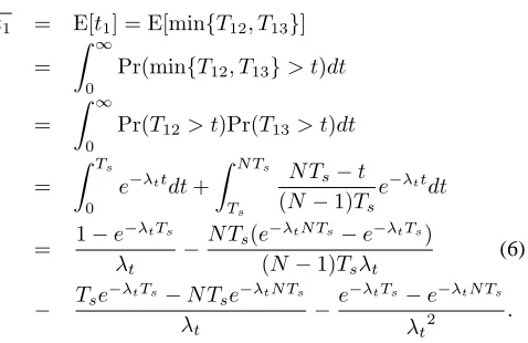
Based on the derived state transition probabilities, the mean residence time of the sensor node in each state is calculated. Similar to the above derivation, we only derive the values of the mean residence time in sleep state and reuse the results obtained in [8] for the other mean residence time values. The mean residence time in the sleep state in AFECA is derived using the newly derived state transition probabilitiesP12and
=
Z ∞
0
Pr(min{T12, T13}> t)dt
=
Z ∞
0
Pr(T12> t)Pr(T13> t)dt
=
Z Ts
0
e−λttdt+ Z N Ts
Ts
N Ts−t
(N−1)Tse −λttdt
= 1−e
−λtTs
λt −
N Ts(e−λtN Ts−e−λtTs)
(N−1)Tsλt (6)
− Tse−λtTs−N Tse−λtN Ts
λt
−e−λtTs−e−λtN Ts
λt2
.
Based on the values ofπk andtk, we can obtain the steady state probability of each sensor node state using Eq. (1) [10]. The energy consumption of a sensor node per unit time is obtained by using the steady state probability as follows:
E=
6
X
k=1
ψkPk, (7)
whereψk is the power consumption in statek.
III. Numerical Examples
For numerical examples, we use the same default parameter values assumed in [8], i.e., Ts= 360010 h, Tl = 360010 h,Ta =
10
3600h, ρ= 0.1, wf = 10, µ1t =
10
3600h, µ1r =
10
3600h, µ1f =
10
3600h, λt = 3600210/h, λr = 360021 /h, λf = 360021 /h, ψ1 =
0.025W, ψ2 = 1.155W, ψ3 = 1.6W, ψ4 = 1.2W, ψ5 =
[image:3.595.313.552.89.244.2]1.6W, andψ6= 1.5W.
[image:3.595.85.293.426.544.2]Figure 4 shows the effect of N for steady state probability of BECA and AFECA. We note that instead of showing the probabilities of four sub-states; transmit, active-receive, active-forward, and active-idle states, respectively, we show the probability of active state collectively, in order to simplify and strengthen the result. Since BECA is irrelevant to N, steady state probabilities of BECA does not change. On the other hand, the probability of sleep state of AFECA increases as the value ofN increases, and the probabilities of other states decreases as the value ofN decreases. As shown in Fig. 5, the energy consumption of AFECA is significantly less than that of BECA and the energy consumption of AFECA decreases as the value ofN increases. However, the rate of decrease of energy consumption of AFECA decreases asN increases, since the probability of sleep state of AFECA saturates as the value of N increases. From Fig. 5, it can be shown that AFECA achieves significant improvement of energy conservation over BECA, even for a small values of N.
0 0.1 0.2 0.3 0.4 0.5 0.6 0.7 0.8 0.9
2 4 6 8 10 12 14 16 18 20
S
te
a
d
y
s
ta
te
p
ro
b
a
b
ili
ty
N
[image:4.595.306.537.75.236.2]Psleep (BECA) Plisten (BECA) Pactive (BECA) Psleep (AFECA) Plisten (AFECA) Pactive (AFECA)
Fig. 4. Steady state probability for varyingN.
0.1 0.2 0.3 0.4 0.5 0.6 0.7 0.8 0.9 1
2 4 6 8 10 12 14 16 18 20
E
n
e
rg
y
C
o
n
s
u
m
p
ti
o
n
(
J
)
N
BECA AFECA
Fig. 5. Energy consumption for varyingN.
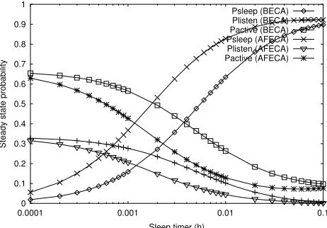
of sleep state of AFECA is larger than that of BECA due to increased sleep timer value, and the probabilities of listen and active states of AFECA are less than those of BECA. Also, we note that the probabilities of the same state in both AFECA and BECA converge to the same value when the value of sleep timer is very large, since the effect of N is negligible for very large value of sleep timer. The energy consumption of AFECA is smaller than that of BECA because of the increased probability of sleep state and decreased probability of listen and active states, as shown in Fig. 7. Also, the energy consumptions of both schemes converge to the same value for very large values of sleep timer, where the effect of N is negligible. Similar to Fig. 5, it is shown that AFECA achieves significant improvement of energy conservation over BECA, even for a small values of N, when the value of sleep timer is not very large.
Figures 8 and 10 show the effect of listen timer and active timer, on the steady state probability, respectively, forN = 5. Figures 9 and 11 show the effect of listen timer and active timer, on the energy consumption, respectively, for varying the values ofN. Similar to Fig. 6, the shape of steady state probabilities of AFECA is very similar to that of BECA in [8], as shown in Figs. 8 and 10, and the probabilities of sleep
0 0.1 0.2 0.3 0.4 0.5 0.6 0.7 0.8 0.9 1
0.0001 0.001 0.01 0.1
S
te
a
d
y
s
ta
te
p
ro
b
a
b
ili
ty
Sleep timer (h)
Psleep (BECA) Plisten (BECA) Pactive (BECA) Psleep (AFECA) Plisten (AFECA) Pactive (AFECA)
Fig. 6. Steady state probability for varying sleep timer.
0 0.2 0.4 0.6 0.8 1 1.2 1.4
0.0001 0.001 0.01 0.1
E
n
e
rg
y
C
o
n
s
u
m
p
ti
o
n
(
J
)
Sleep timer (h)
[image:4.595.305.538.268.431.2]BECA AFECA (N=2) AFECA (N=5) AFECA (N=10) AFECA (N=20)
Fig. 7. Energy consumption for varying sleep timer.
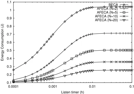
state in AFECA are larger than those in BECA. Therefore, the energy consumption of AFECA is smaller than that of BECA, as shown in Figs. 9 and 11. We note that the steady state probability of all the states of both schemes saturates for large values of sleep timer since there is few transition from listen to sleep state, and thus, energy consumption of both schemes also saturate. In Fig. 11, on the other hand, the energy consumptions of both schemes converge to the same value for very large values of active timer, where the effect of N is negligible since states remain in active state almost always. Similar to Figs. 5 and 7, it is shown that AFECA achieves significant improvement of energy conservation over BECA, even for a small values of N, when the values of active timer are not very large.
IV. Conclusions and Further Works
[image:4.595.47.280.269.436.2]0 0.1 0.2 0.3 0.4 0.5 0.6 0.7 0.8
0.0001 0.001 0.01 0.1
S
te
a
d
y
s
ta
te
p
ro
b
a
b
ili
ty
Listen timer (h)
[image:5.595.303.538.72.237.2]Psleep (AFECA) Plisten (AFECA) Pactive (AFECA)
Fig. 8. Steady state probability for varying listen timer.
0.1 0.2 0.3 0.4 0.5 0.6 0.7 0.8 0.9 1 1.1
0.0001 0.001 0.01 0.1
E
n
e
rg
y
C
o
n
s
u
m
p
ti
o
n
(
J
)
Listen timer (h)
BECA AFECA (N=2) AFECA (N=5) AFECA (N=10) AFECA (N=20)
Fig. 9. Energy consumption for varying listen timer.
of BECA in detail. The results show that AFECA achieves significant improvement of energy conservation over BECA, even for a small values ofN, when the values of sleep timer and active timer are not very large. The result of this paper can provide sensor network operators guideline for selecting appropriate timer values for AFECA.
We note, however, that the reduction of energy consumption in AFECA is possible, at the expense of increased packet delivery delay due to increased probability of sleep state. In our further works, the increased packet delivery delay in AFECA will be investigated analytically in detail, based on the estimation of the number of neighboring nodes and traffic characteristics. Also, an adaptive algorithm for select-ing either BECA or AFECA, dependselect-ing on the quality of service (QoS) requirement of requested packet delivery, will be proposed and analyzed as our further works, too.
References
[1] I. F. Akyildiz, W. Su, Y. Sankarasubramaniam, and E. Cayirci, “A survey on sensor networks,” IEEE Commun. Mag., vol. 40, pp. 102-114, 2002.
[2] J. Yick, B. Mukherjee, and D. Ghosal, “Wireless sensor network survey,” Elsevier Comput. Netw., vol. 52, pp. 2292-2330, 2008.
0 0.2 0.4 0.6 0.8
0.0001 0.001 0.01 0.1
S
te
a
d
y
s
ta
te
p
ro
b
a
b
ili
ty
Active timer (h)
[image:5.595.48.279.73.238.2]Psleep (AFECA) Plisten (AFECA) Pactive (AFECA)
Fig. 10. Steady state probability for varying active timer.
0 0.2 0.4 0.6 0.8 1 1.2 1.4 1.6
0.0001 0.001 0.01 0.1
E
n
e
rg
y
C
o
n
s
u
m
p
ti
o
n
(
J
)
Active timer (h)
BECA AFECA (N=2) AFECA (N=5) AFECA (N=10) AFECA (N=20)
Fig. 11. Energy consumption for varying active timer.
[3] N. A. Pantazis and D. D. Vergados, “A Survey on Power Control Issues in Wireless Sensor Networks,” IEEE Comm. Surveys and Tutorials, vol. 9, pp. 86-107, 2007.
[4] G. Anastasi, M. Conti, M. D. Francesco, and A. Passarella, “Energy conservation in wireless sensor networks: a survey,” Elsevier Ad Hoc Networks, vol. 7, pp. 537-568, 2009.
[5] A. Savvides, C. C. Han, and M. Srivastava, “Dynamic fine-grained localization in ad-hoc networks of sensors,” In Proceedings of the ACM SIGMOBILE Annual International Conference on Mobile Computing and Networking, Rome, Italy, pp. 166-179, July 2001.
[6] C. E. Jones, K. M. Sivalingam, and P. Agrawal, J. C. Chen, “A survey of energy efficient network protocols for wireless networks,” Wirel. Netw., vol. 7, pp. 343-358, 2001.
[7] Y. Xu, J. Heidemann, and D. Estrin, “Adaptive energy-conservation routing for multi-hop ad hoc networks,” Technical Report 527, USC/Informaton Sciences Institute, 2000.
[8] Y. W. Chung and H. Y. Hwang, “Modeling and analysis of energy conservation scheme based on duty cycling in wireless ad hoc sensor network, Sensors, vol. 10, no. 6, pp. 5569-5589, June. 2010. [9] Q. Gao, K. J. Blow, D. J. Holding, I. Marshall, “Analysis of energy
conservation in sensor networks,” Wirel. Netw., vol. 11, pp. 787-794, 2005.
[image:5.595.303.539.269.433.2] [image:5.595.46.280.270.434.2]