Application of Bootstrap in Dose Apportionment of Nuclear Plants Via Uncertainty Modeling of the Effluent Released from Plants

Application of Bootstrap in Dose Apportionment of

Nuclear Plants via Uncertainty Modeling of the Effluent

Released from Plants

Debabrata Datta

Health Physics Division, Bhabha Atomic Research Centre, Mumbai, India Email: [email protected]

Received May 20, 2011; revised July 2, 2011; accepted August 25, 2011

ABSTRACT

Nuclear power plants are always operated under the guidelines stipulated by the regulatory body. These guidelines ba- sically contain the technical specifications of the specific power plant and provide the knowledge of the discharge limit of the radioactive effluent into the environment through atmospheric and aquatic route. However, operational con- straints sometimes may violate the technical specification due to which there may be a failure to satisfy the stipulated dose apportioned to that plant. In a site having multi facilities sum total of the dose apportioned to all the facilities should be constrained to 1 mSv/year to the members of the public. Dose apportionment scheme basically stipulates the limit of the gaseous and liquid effluent released into the environment. Existing methodology of dose apportionment is subjective in nature that may result the discharge limit of the effluent in atmospheric and aquatic route in an adhoc manner. Appropriate scientific basis for dose apportionment is always preferable rather than judicial basis from the point of harmonization of establishing the dose apportionment. This paper presents an attempt of establishing the dis- charge limit of the gaseous and liquid effluent first on the basis of the existing value of the release of the same. Existing release data for a few years (for example 10 years) for any nuclear power station have taken into consideration. Boot- strap, a resampling technique, has been adopted on the existing release data sets to generate the corresponding popula- tion distribution of the effluent release. Cumulative distribution of the population distribution obtained is constructed and using this cumulative distribution, 95th percentile (upper bound) of the discharge limit of the radioactive effluents is computed. Dose apportioned for a facility is evaluated using this estimated upper bound of the release limit. Paper de- scribes the detail of the bootstrap method in evaluating the release limit and also presents the comparative study of the dose apportionment using this new method and the existing adhoc method.

Keywords: Dose Apportionment; Radioactive; Effluent; Cumulative Distribution; Bootstrap; Percentile

1. Introduction

During the normal operation of any nuclear facility gase- ous and liquid radioactive effluents are routinely discharged into the environment. These can result in radiation dose to the members of the public through various exposure path- ways. Regulatory authority (for example, Atomic Energy Regulatory Board in India) in line with the International Commission of Radiological Protection (ICRP), has pre- scribed an effective dose limit of 1 mSv/y for a member of the public which requires routine radioactive release to be authorized or stipulated within a limit. The objective of dose apportionment of the nuclear facilities including power plants, fuel reprocessing plant and waste immobi- lization plant is to establish the discharge limit of the ga- seous and the liquid radioactive effluents into the envi- ronment so that the dose received by the members of the public will be 1 mSv/year. In India, the operating Nuclear

of these radioactive effluents is an issue of ensuring safety of the facility as well as safety of the environment. The existing discharge limits for the NPPs were established when the nuclear power program was at its initial stages. However, expansion program of nuclear power in the coun- try demands the dose apportionment to be revisited in an appropriate scientific manner, so that release limits for the existing plants can be revised and the same for new plants to be installed at the same site can be established with the similar vintage. Statistical analysis of the existing dis- charge (gaseous and liquid effluents) data from the facil- ity is taken into account to establish the release limit of that facility. Statistical analysis is carried out using boot- strap technique because of the imprecise structure of the release data. This paper presents the detail of bootstrap methodology [1] of arriving at the radioactive effluent re- lease limits of Indian Nuclear Power Plants (NPPs). Boot- strap method of estimation of the discharge limits of the gaseous and liquid effluents also provides the knowledge of the cumulative distribution of the discharge. Cumula- tive distribution of the gaseous and liquid effluent dis- charge is used to estimate the uncertainty of the same and the uncertainty is expressed in the form of 5th and 95th percentiles. Uncertainty estimate of the discharges can be used in a standard dose assessment model to compute the uncertainty of the apportioned dose to a specific facility. Recommendation of dose apportionment can be finally be made with its 95th percentile value. Computation has been carried out using a computer code developed in house using Visual Basic 6.0.

2. Regulatory Control of Radioactive

Discharge

Establishment of dose apportionment of a nuclear install- lation is one of the important safety aspects in the sense that the task of dose apportionment will automatically pro- vide the setting the limit of the discharge of the effluent both in the atmospheric and aquatic route. On the other hand, it will also provide the knowledge of how many more nuclear facilities can be possible to install at the same site. Dose apportionment scheme should follow the basic cri- teria as: the sum total of “dose apportionment of new facility”, “dose apportionment of old facility” and “the re- serve” should be altogether equal to 1 mSv. In order to achieve this one has to set the appropriate limit of the dis- charge of the radioactivity into the atmospheric and aquatic environment. Recent work on the development of standards for the radioactive discharge control includes the devel- opment of practical guidance for setting discharge limits. ICRP Publication 60 [2] recommends justifying necessary measures for protection of the public in practice situations via constrained optimization procedures [3]. Public annual effective dose limit from all controllable environmental radiation sources (except of natural background) was al-

ready established as equal to 1 mSv. Accordingly, the con- straint value relevant to a single source should be a non- specified fraction of this limit. Both the dose limit and constraint apply to representatives of the highest exposed members of the public (the critical group) in the radiation conditions under consideration. According to the relevant Safety Fundamentals [4], “The objective of radioactive waste management is to deal with radioactive waste in a manner that protects human health and the environment now and in the future without imposing undue burdens on future generations.”

3. Bootstrap Method

Bootstrap procedures are robust nonparametric statistical methods that can be used to construct approximate confi- dence limits for the population mean, to estimate the bias and variance of an estimator or calibrate hypothesis tests [5]. In these procedures, repeated samples of size n are drawn with replacement from a given set of observations. The process is repeated a large number of times (e.g., thou- sands), and each time an estimate of the desired unknown parameter (e.g., the sample mean) is computed. Details of bootstrap and the diversity of its recent applications can be found elsewhere [5-9]. Bootstrap procedures assume only that the sample data are representative of the under- lying population. The bootstrap procedures require no as- sumptions regarding the statistical distribution (e.g., nor- mal, lognormal, gamma) of the underlying population and can be applied to a variety of situations [10]. However, since they involve extensive resampling of the data and, thus, exploit more of the information in a sample, that sam- ple must be a statistically accurate characterization of the underlying population in all respects (not just in its mean and standard deviation). Therefore, the bootstrap methods are specifically useful when: the exact population distribu- tions of the statistics are not known; or the critical values of the test statistics are not available; Bootstrap procedures are classified as (a) standard bootstrap, (b) bootstrap-t, (c) bias corrected accelerated (BCA) bootstrap and (d) per- centile bootstrap [10]. In practice, it is random sampling that satisfies the representativeness assumption. There- fore the data must represent random samples of the under- lying population. If sample size is small and the distribu- tion is not known exactly bootstrap application on that sam- ple generates the corresponding population and the popu- lation can be used to compute the upper confidence limit (UCL) of the population distribution. Bootstrapping pro- cedures are inappropriate for use with data that were idio- syncratically collected or focused especially on contami- nation hot spots. Algorithm of bootstrap used for computing upper confidence limit (UCL) [11] is written below:

Algorithm:

Let X1, X2, ···, Xn represent the n randomly sampled

Step1: Compute the sample mean:

1

1 n

i i

X X

n 





Step 2: Compute the sample standard deviation:





1 n

i i

s X X

n 





Step 3: Compute the sample skewness:





1

1 n

i i

k X

ns 





Step 4:For b = 1 to B (a very large number) do the fol- lowing:

1) Generate a bootstrap sample data set; i.e.,

for i = 1 to n let j be a random integer between 1 and n and add observation Xjto the bootstrap sample data set.

2) Compute the arithmetic mean X_b of the data set constructed in step 1.

3) Compute the associated standard deviation sbof the

constructed data set.

4) Compute the skewness kbof the constructed data

using the formula in step 3.

5) Compute the studentized mean





6) Compute Hall’s statistic:

2 2 3

3 27

b b b

Q W k W  k W k 6n

Step 5: Sort all the Q values computed in Step 4 and select the lower αth quantile of these B values. It is the (αB)th value in an ascending list of Q’s. This value is from the left tail of the distribution.

Step 6: Compute

   













3 1 6 1

W Q  k k Q_k n 

Step 7: Compute the one-sided (1-α) confidence limit on the mean.

 

UCL_ X W Q s _

4. Mathematical Background of Dose

Apportionment

4.1. Atmospheric Discharges

The dose apportionment methodology is basically a scheme to compute the dose to the member of the public at exclu- sion distance (1.6 km from location of the plant) corre- sponding to the discharge limit of the radioactive gaseous and liquid effluent released due to routine operation of the facility. This estimated dose should be a fraction of the limit 1 mSv/yr as stipulated by the regulatory authority. Discharge limit is considered as the technical specification limit of the discharge. Operational experience reveals that the actual discharge is always far below the technical spe-

cification as set up during the design of the plant. With a view to this fact, it is obvious that if we properly assess the discharge limit based on the operating experience of the facility, we can have the corresponding apportioned dose in a better perspective in the sense that we can have a sub- stantial margin to reach at 1 mSv/yr limit resulting the pro- vision of installation of some more new nuclear power plants or other nuclear facilities. Standard environmental dose assessment model along with the site-specific me- teorological data and dietary intake data are used for the computation of dose. The dose to the members of the pub- lic can be mathematically formulated as





,

1 1

Dose Dose 1 mSv yr

n n

k p k aquatic p k _air k

 

 

 







where, the index “p” denotes the pathways of exposure and the index “k” denote the radionuclide. Figure 1 gives the block diagram for the main steps in arriving at tech- nical specification limits and dose apportionment. The dose received by the members of public is computed for all re- levant pathways of exposure. The dose apportionment of fission product noble gas (FPNG) and Ar-41 is based on the dose versus release relationship and the Technical Spe- cification limits for discharge. Mathematically the appor- tioned dose to FPNG and Ar-41 nuclide can be formu- lated as











_{ }



Bq d mSv y per Bq s Appdos mSv y

8.64 10 s d

DCF

 





(2) where,  is Tech spec limit and the other symbols have usual significance. The computation of plume doses in 22.5˚ sector from continuous release of noble gases (Ar-41 and fission product noble gases) can be found elsewhere in [12]. The sector receiving the highest dose is called as the

critical sector and subsequently sector average dose is used for computation for dose apportionment [12]. Accordingly, contributions from the adjacent two side sectors, on either side of main sector, are also consider to arrive at a rela- tionship between release rate and dose at exclusion dis- tance. The gamma energy used for computation is 1.28 MeV for Ar-41 and 0.65 MeV for a mixture of Xenon and Krypton isotopes. In order to compute the site specific relationship between release rate and dose the frequency (f)/wind speed (u) (m/s)) for the main sector and the two side sectors are used with which the dose rates are mul- tiplied. Finally all these results are summed up for all wea- ther categories [12]. The dose apportionment for internal irradiators like H-3, I-131 and particulates can be written mathematically as







 















 

3

3

DoseApp mSv y

Bq d s m

DAC pub Bq m mSv y 8.64 10 s d

X Q

 



  4

(3)

where,  is Tech spec limit, DAC (pub) is the derived air concentration applicable to members of the public corre- sponding to dose limit of 1 mSv/y and X/Q is the annual average atmospheric dilution factor at the exclusion dis- tance for the critical sector. The X/Q value applicable for the particular stack height at a distance of 1.6 km from the stack and corresponding to the critical sector is used in the calculation of dose apportionment. The derived air concentration (DAC, public) is defined as the ground le- vel air concentration of radionuclides that results the ef- fective dose limit of 1 mSv/y to members of the public from all-important pathways of exposure. The DAC (pub- lic) is generally calculated for both adult and infants and the more restrictive of the two are generally used for cal- culation of the derived limits. The computation of dose for tritium in detail is depicted elsewhere [12].

4.2. Aquatic Discharges

The dose apportionment for radionuclides discharged into the aquatic environment is computed from the technical specifications limit on concentration for gross beta and Tritium. Mathematical models used in dose apportionment for gross beta for the coastal site and for the inland site are given by













   

Dose appor mSv y Coastal site

Conc tech spec Bq ml *I_f* CF _i DF P_{i i}

  (4)

where, If is the annual intake of fish by the population for

a given NPP site, (g/y), CFiis the concentration factor in

marine fish for radionuclide i (ml/g), DFi is the inges-

tion dose conversion factor for ith radionuclide (Sv/Bq),

Pi is the percentage composition of ith radionuclide in the

gross activity.













   

Dose appor mSv y Inland site

Conc tech spec Bq ml * Iw I x CFf i DF i

 _  _ P_i

(5) where, Iwis the annual intake of drinking water (ml/y), If

is the annual intake of fish by the population for a given NPP site (g/y), CFi is the concentration factor in marine

fish for ith radionuclide, DFiis the ingestion dose conver-

sion factor for ith radionuclide (Sv/Bq), Pi is the percent-

age composition of ith radionuclide in the gross activity.

5. Bootstrap Method in Dose Apportionment

appropriate limit for establishing the dose apportionment of various nuclear power stations.

6. Results and Discussion

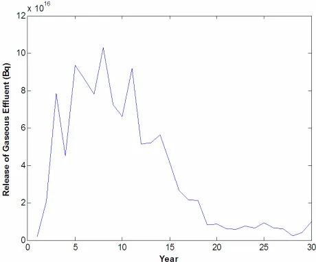
The operating experience of a typical plant #1(considered as an installation in the coastal site) is represented in the form of actual yearly release of gaseous and liquid efflu- ent and the same dataset is as presented in Table 1 and

Table 2 respectively. The corresponding distribution of the gaseous and liquid effluent released from the specific nuclear power plant is as shown in Figures 1 and 2. It can be easily investigated from Figures 1 and 2 that arithme- tic mean or simple average of the actual release is not the representative input for the estimation of the dose appor- tioned for the specified nuclide for that specific plant be- cause the shape of distribution of the release data is not the normal distribution. It is confirmed by carrying out the normality test (Kolmogorov-Smirnov Test) [20] of the re- presented data (Tables 1 and 2); the test fails confirming that the distribution of these data is not normal. Moreover,

Table 1. Yearly actual release values of gaseous effluent (plant #1).

Year Total (Bq) Year Total (Bq) Year Total (Bq) 1 1.9E+15 11 9.19E+16 21 6.04E+15 2 2.08E+16 12 5.13E+16 22 5.94E+15 3 7.84E+16 13 5.2E+16 23 7.63E+15 4 4.52E+16 14 5.62E+16 24 6.35E+15 5 9.36E+16 15 4.14E+16 25 9.41E+15 6 8.63E+16 16 2.66E+16 26 6.56E+15 7 7.82E+16 17 2.15E+16 27 6.12E+15 8 1.03E+17 18 2.11E+16 28 2.34E+15 9 7.23E+16 19 8.11E+15 29 4.14E+15 10 6.6E+16 20 8.48E+15 30 1.01E+16

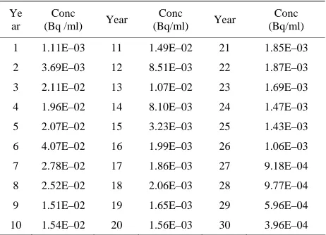
Table 2. Yearly actual release values of liquid effluent from a typical plant #1.

Ye ar

Conc

(Bq /ml) Year

Conc

(Bq/ml) Year

Conc (Bq/ml) 1 1.11E–03 11 1.49E–02 21 1.85E–03 2 3.69E–03 12 8.51E–03 22 1.87E–03 3 2.11E–02 13 1.07E–02 23 1.69E–03 4 1.96E–02 14 8.10E–03 24 1.47E–03 5 2.07E–02 15 3.23E–03 25 1.43E–03 6 4.07E–02 16 1.99E–03 26 1.06E–03 7 2.78E–02 17 1.86E–03 27 9.18E–04 8 2.52E–02 18 2.06E–03 28 9.77E–04 9 1.51E–02 19 1.65E–03 29 5.96E–04

10 1.54E–02 20 1.56E–03 30 3.96E–04

Figure 2. Distribution of yearly release of liquid effluent from plant #1.

the represented data being a time series one cannot simply take the mean without appropriate trend analysis. In order to overcome this difficulty, bootstrap method has been ap- plied on the data set to construct the population distribu- tion associated with the represented data. The frequency distribution of the release data after bootstrap (histogram) is shown in Figure 3 and corresponding cumulative dis- tribution plot is as shown in Figure 4. Cumulative dis- tribution provides the knowledge of 5th and 95th percen-tiles of the probability density of release data set. Upper confidence limit as 95th percentiles estimated from un- certainty analysis of the effluent released data is accepted as the appropriate input for dose apportionment calcula- tion Figures 5 and 6 represent the frequency distribution (histogram) and the corresponding cumulative distribu- tion of the gross beta release from plant #1. Cumulative distribution is then utilized to estimate the 5th, 50th and 95th percentiles of the release of the gaseous and liquid effluents from the plant #1.

Figure 3. Population distribution of FPNG release from plant #1 after bootstrap (sample size of bootstrap: 100,000).

Figure 4. Cumulative distribution of FPNG release from plant #1.

Figure 5. Population distribution of gross beta release from plant #1 after bootstrap (bootstrap sample size taken: 100,000).

Figure 6. Cumulative distribution of gross beta release from plant #1.

Table 3. Uncertainty estimate of gaseous and liquid effluent release from plant #1.

Release per Year 5thPercentile 50th Percentile 95th Percentile

FPNG (Bq) 2.66E16 3.62E16 4.64E16

Gross Beta (Bq/ml) 0.0053 0.0080 0.0111

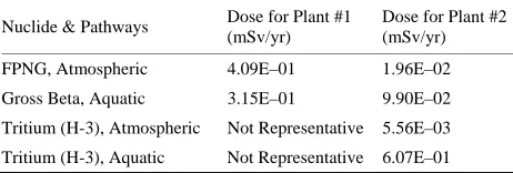
into consideration for this case study. Uncertainty estimates for distribution of each radionuclide using same method- ology are tabulated in Table 4. Site specific value of the at- mospheric average dilution factor (X/Q), Condenser cooling water (CCW) flow for dilution in the aquatic route, DAC (public), composition of radionuclide for gross beta, con- centration factors, intake of fish and the drinking water are used as input for dose calculation. All the required in- put parameters are listed in Table 5. Apportioned dose using the input parameters listed in Table 5 and 95th percentile value of FPNG and Gross Beta from plant #1 (coastal site) and that of FPNG, H-3 (air), H-3 (liquid) and gross beta from plant #2 are computed and the results are tabulated in Table 6. Comparative study of the dose apportioned for plant #1 and plant #2 from Table 6 indi- cate that apportioned dose for FPNG and gross beta for plant at coastal site is more than for plant at inland site. Tritium in air and in aquatic environment for plant #1 is not representative because plant #1 is of boiling water type nuclear reactor.

7. Conclusion

Table 4. Uncertainty estimate of Gaseous and Liquid Effluent Release from Plant #2.

Release 5th Percentile 50th Percentile 95th Percentile

FPNG (Bq/d) 1.08E13 1.97E13 3.42E13

H-3 (Air) (Bq/d) 0.77E13 1.58E13 2.96E13

H-3 (Liquid) (Bq/ml) 13.77 21.05 30.7

Gross Beta (Bq/ml) 0.002 0.003 0.004

Table 5. Input Parameters used for dose computation.

Parameters Plant #1 (Coastal) Plant #2 (Inland) Atmospheric average

dilution factor (s/m3₎ 6.92E–8 5.34E–8

CCW flow (m3/day) 2.90E+06 44880

DAC, public (Bq/m3_{) Not representative 3294} Intake of fish (g/yr) 20000 3000 Intake of water (litre/yr) Not representative 1.10E3

Concentration factors of important radionuclide

22 (Cs-137, Cs-134), 11.3(Sr-90), 4200 (Co-60)

13.2 (Cs-137,Cs-134), 300 (Co-60), 600 (Zn-65)

Table 6. Computed Apportioned Dose for Plant #1 and Plant #2.

Nuclide & Pathways Dose for Plant #1 (mSv/yr)

Dose for Plant #2 (mSv/yr)

FPNG, Atmospheric 4.09E–01 1.96E–02

Gross Beta, Aquatic 3.15E–01 9.90E–02 Tritium (H-3), Atmospheric Not Representative 5.56E–03 Tritium (H-3), Aquatic Not Representative 6.07E–01

tile value is used as the discharge limit of the effluent and using this 95th percentile as an input to the standard dose assessment model, dose computation has been carried out. Final conclusion is that bootstrap provides a scientific basis of dose apportionment scheme. It can be further concluded that uncertainty analysis of the effluent data only is essen- tial for estimating the apportioned dose to a nuclear facil- ity. However, an optimization approach is essential when dose apportionment is required for many more plants lo- cated at the same site. Research is being continued to de- velop an optimization technique for this purpose.

REFERENCES

[1] B. Efron and R. J. Tibshirani, “An Introduction to the Bootstrap,” Chapman and Hall, New York, 1993.

[2] “International Commission on Radiological Protection, 1990 Recommendations of the International Commission on Radiological Protection,” ICRP Publication 60, Per- gamon Press, Oxford and New York, 1991.

[3] M. Balonov, G. Linsley, D. Louvat, C. Robinson and T.

Cabianca, “The IAEA Standards for the Radioactive Dis- charge Control: Present Status and Future Development,” Radioprotection, Vol. 40, Suppl. 1, S721-S726, 2005. doi:10.1051/radiopro:2005s1-105

[4] International Atomic Energy Agency, “Regulatory Con- trol of Radioactive Discharges to the Environment,” Sa- fety Standards Series No. WS-G-2.3, IAEA, Vienna, 2000.

[5] M. R. Chernick, “Bootstrap Methods, A Practitioner’s Guide,” Wiley, New York, 1999.

[6] P. Hall, “The Bootstrap and Edgeworth Expansion,” Sprin- ger-Verlag, New York, 1992.

[7] G. Archer and J. M. Giovannoni, “Statistical Analysis with Bootstrap Diagnostics of Atmospheric Pollutants Pre- dicted in the APSIS Experiment,” Water, Air, and Soil Pollution, Vol. 106, No. 1-2, 1998, pp. 43-81.

doi:10.1023/A:1005004022883

[8] A. C. Davison and D. V. Hinkley, “Bootstrap Methods and Their Application,” Cambridge University Press, Cambri- dge, 1997.

[9] B. Efron, “The Jackknife, the Bootstrap and Other Resam- pling Plans,” SIAM, Philadelphia, 1982.

doi:10.1137/1.9781611970319

[10] E. J. Dudewicz, “The Generalized Bootstrap,” In: K.-H. Jöckel, G. Rothe and W. Sendler, Eds., Bootstrapping and Related Techniques, Springer-Verlag, Berlin, 1992, pp. 31-37.

[11] T. J. DiCiccio and B. Efron, “Bootstrap Confidence Inter- vals (with Discussion),” Statistical Science, Vol. 11, No. 3, 1996, pp. 189-228.

[12] International Atomic Energy Agency, “Generic Models for Use in Assessing the Impact of Discharges of Radio- ac-tive Substances to the Environment,” Safety Reports Se-ries No. 19, IAEA, Vienna, 2001.

[13] International Atomic Energy Agency, “Basic Safety Stan- dards Series,” SS No. 115, IAEA, Vienna, 1996.

[14] A. J. Bailer and J. T. Oris, “Assessing Toxicity of Pollut- ants in Aquatic Systems,” In: N. Lange, L. Ryan, L. Billard, D. Brillinger, L. Conquest and J. Greenhouse, Eds., Case Studies in Biometry, Wiley, New York, 1994, pp. 25-40. [15] R. L. Cooley, “Confidence Intervals for Groundwater Mo-

dels Using Linearization, Likelihood, and Bootstrap Me- thods,” Ground Water, Vol. 35, No. 5, 1997, pp. 869-880. doi:10.1111/j.1745-6584.1997.tb00155.x

[16] J. S. U. Hjorth, “Computer Intensive Statistical Methods —Validation Model Selection and Bootstrap,” Chapman and Hall, New York, 1994.

[17] C. Davison and D. Y. Hinkley, “Bootstrap Methods and Their Application,” Cambridge University Press, Cambri- dge, 1997.

[18] R. LePage and L. Billard, “Exploring the Limits of Boot- strap,” John Wiley, New York, 1992.

[19] P. Barbe and P. Bertail, “The Weighted Bootstrap (Lec-ture Notes in Statistics),” Springer-Verlag, New York, 1995.