Centrality Measures Based on Matrix Functions

(1)

ISSN Online: 2161-7643 ISSN Print: 2161-7635

DOI: 10.4236/ojdm.2018.84008 Sep. 26, 2018 79 Open Journal of Discrete Mathematics

Centrality Measures Based on Matrix Functions

Lembris Laanyuni Njotto

Department of Mathematics and ICT, College of Business Education, Dar Es Salaam, Tanzania

Abstract

Network is considered naturally as a wide range of different contexts, such as biological systems, social relationships as well as various technological scena-rios. Investigation of the dynamic phenomena taking place in the network, determination of the structure of the network and community and descrip-tion of the interacdescrip-tions between various elements of the network are the key issues in network analysis. One of the huge network structure challenges is the identification of the node(s) with an outstanding structural position within the network. The popular method for doing this is to calculate a measure of centrality. We examine node centrality measures such as degree, closeness, eigenvector, Katz and subgraph centrality for undirected networks. We show how the Katz centrality can be turned into degree and eigenvector centrality by considering limiting cases. Some existing centrality measures are linked to matrix functions. We extend this idea and examine the centrality measures based on general matrix functions and in particular, the logarith-mic, cosine, sine, and hyperbolic functions. We also explore the concept of generalised Katz centrality. Various experiments are conducted for different networks generated by using random graph models. The results show that the logarithmic function in particular has potential as a centrality measure. Simi-lar results were obtained for real-world networks.

Keywords

Graph, Centrality Measures, Matrix Functions, Kendall Correlation Coefficient, Random Graph Models

1. Introduction

Since its introduction by Euler in eighteen century, graph theory has proven its important applications in many different scientific fields. Graphs and linear al-gebra have been used to model social interactions. Recently network models are now commonplace not only in the hard sciences but also in various

technologi-How to cite this paper: Njotto, L.L. (2018) Centrality Measures Based on Matrix Func-tions. Open Journal of Discrete Mathemat-ics, 8, 79-115.

https://doi.org/10.4236/ojdm.2018.84008 Received: July 12, 2018

Accepted: September 23, 2018 Published: September 26, 2018 Copyright © 2018 by author and Scientific Research Publishing Inc. This work is licensed under the Creative Commons Attribution International License (CC BY 4.0).

(2)

DOI: 10.4236/ojdm.2018.84008 80 Open Journal of Discrete Mathematics

cal, social and biological scenarios. Networks are used to model a variety of highly interconnected systems, both in nature and man-made world of technol-ogy. These networks include protein-protein interaction networks, social net-works, food webs, scientific collaboration netnet-works, metabolic netnet-works, lexical or semantic networks, neural networks, the World Wide Web and others. The use of network analysis is in various situations: from determining network structure and communities, describing the interactions between various ele-ments of the network and investigating the dynamics phenomena taking place in the network [1].

One of the ground laying questions analysis of network is how to determine the “most important” nodes in a given network. Many centrality measures have been proposed, starting with the simplest of all, node degree centrality. This measure has being considered too “local”, as it does not take into account the connectivity of the immediate neighbours of the node under consideration. A number of centrality measures have been introduced that take into account the global connectivity properties of the network. These include various types of ei-genvector centrality for both directed and undirected networks, Katz centrality, subgraph centrality and PageRank centrality [1]. The use of centrality scores provides rankings of the nodes in the networks. The higher the ranking of a node, the more important the node is believed to be within the network. There are many different ranking methods in use, and many algorithms have been de-veloped to compute these rankings.

The purpose of this paper is to discuss some of the centrality measures and analyse the relationship between degree centrality, eigenvector centrality, and Katz centrality and to discuss the measures of centrality based on matrix tions including the logarithmic, sine, cosine, exponential and hyperbolic func-tion. The main aim is to determine which of the matrix functions is highly cor-related to “standard” centrality measures. We will use the Kendall correlation coefficient [2] in the experimental work to determine the correlations.

2. Literature Review

Bavelas [3] introduces the application of centrality of networks in human com-munication by measuring the comcom-munication within a small group in terms of the relationship between the structural centrality and influence in a group process. Afterwards, an application of centrality was made under the direction of Bavelas at the Group Networks Laboratory, M.I.T in the late 1940s. Leavitt in 1949 and Smith in 1950 conducted a study on centrality measure on which Ba-velas in 1950 and BaBa-velas and Barrett in 1951 reported. These experiments all concluded that centrality was related to group efficiency in problem-solving and agreed with the subjective perception of leadership [4].

(3)

con-DOI: 10.4236/ojdm.2018.84008 81 Open Journal of Discrete Mathematics

sequences of centrality in communication paths for urban development [6]. Lat-er, Czepiel used the concept of centrality to explain the pattern of diffusion of a technological innovation in the steel industry [7].

Recently, Bolland analysed the stability of the degree (DC), closeness (CC), betweenness (BC), and eigenvector (EC) centrality in random and systematic variations of network structure, and found that betweenness centrality changes significantly with the variation of the network structure, while degree and close-ness centrality are usually stable. He also found that eigenvector centrality is the most stable of all the indices analysed [8]. Borgatti and Frantz extended the stu-dies on the stability of centrality indices by considering the addition and deletion of nodes and links [9] as well as by differentiating several types of network to-pology such as uniformly random, small-world, core-periphery, scale-free, and cellular. Landherr reviewed critically the role of centrality measure in social networks [10]. Estrada analysed examples of how a particular centrality measure is applied in social networks [11].

Benzi and Klymko analysed centrality measures, such as degree, eigenvector, Katz and subgraph for both undirected and directed networks. They used the local and global influence of a given node in the network as measured by walks of different lengths through that node. They analysed the relationship between centrality measures based on the diagonal entries and row sums of the matrix exponential and resolvent of the adjacency matrix involving the degree and ei-genvector centrality. They showed experimentally that the rankings produced by exponential subgraph centrality, total communicability and resolvent subgraph centrality converge to those produced by degree centrality [1].

Most of the centrality measures notations considered are combinatorial in nature and based on the discrete structure of the underlying networks. We can extend our studies by defining the centrality measure by using the spectral techniques from linear algebra. Benzi and Klymko considered the diagonal entries of the matrix exponential f

( )

_A =eA _{and the Katz function}

( ) (

)

1

f α −

= −

A I A where

α

>0_and A is the adjacency matrix of the network [1]. Though, none of the previous studies considered other matrix functions such as the logarithmic, cosine, sine, hyperbolic functions and the generalized Katz centrality as centrality measures. In this work we will develop the notions of centrality based on matrix functions, and we will use the Kendall correlation coefficient [2] to determine the agreement between the node rankings produced by these matrix functions and those produced by the standard centrality measures.

3. Elements of Graph

(4)

An edge starting and ending at the same vertex is called a loop.

• _{Graphs can be represented by using points as nodes (vertices) and joining}

them using line segments for edges. We write uv to denote an edge between nodes u and v.

• _{We can assign numerical values to the edges of a graph in which case the}

graph is referred to as weighted. In an unweighted graph we assign to every edge the value 1.

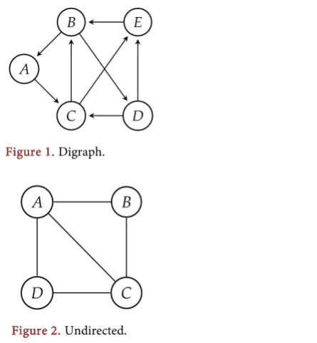
• _{If the edges of the graph are directed (}_{Figure 1}_{), then the graph is called a}

directed graph or digraph otherwise it is called an undirected graph. An undirected unweighted (Figure 2) graph without loops is simple if no two edges connect the same pair of vertices.

• _{For undirected graphs, if there are multiple edges between a pair of nodes}

then the graph is called a multi-graph or pseudo-graph. In digraphs we can have two edges connecting two vertices.

3.1. Basic Graph-Theoretic Terminology

If uv E∈ _{is an edge in an undirected graph}_G_{, then nodes}_u_and_v_{are incident}

to the edge uv and we say that u and v are adjacent (neighbours) in G. It follows that u and v are the endpoints of an edge uv. If G is the directed graph and uv E∈ _{, then}_u_{is said to be adjacent to}_v_and_v_{is said to be adjacent from}_u_{. We}

call u the initial node of uv and v the terminal or end node of uv. For an undirected graph G, the degree deg v

( )

i of a node vi is the total number of

edges which are incident to the corresponding node vi.

The degree deg v

( )

i is the number of “immediate neighbours” of a node vi

in G. In a regular graph all nodes have the same degree. Nodes in directed graphs have an in-degree and an out-degree. The in-degree of a node vi,

( )

i

deg v− _{, is the total number of edges with}

i

[image:4.595.316.539.487.728.2]

v as their terminal node. Similarly,

Figure 1. Digraph.

(5)

the out-degree of vi, deg v+

( )

i , is the total number of edges with vi as their

initial node. Loops contribute 1 to both the in-degree and out-degree.

A graph H=

(

(

,

)

k

W = V E _{of the form}

{

0, , ,1 k

}

, V = v v v

(

) (

)

(

)

{

0, 1 , ,1 2 , , k 1, k

}

E= v v v v  v− v

where vi and vi+1 are adjacent.

A trail in G is a walk in which no edges of G appear more than once (a walk with all different edges). A trail which begins and ends at the same node is known as a closed trail or circuit.

A path in G is a walk in which no nodes appear more than once with the exception that vk can be equal to v0. A cycle or a closed path is a path which

begins and ends at the same node.

Two nodes vi and vj in G are connected if there is a path between them.

We say that graph G is connected if for every pair of nodes vi and vj there

exists a path that starts at vi and ends at

v

j . An edge v vi j∈E in a

connected graph G=

(

V E,

)

_{is a bridge if}_G_{becomes disconnected if}v v_{i j} is deleted. If vi and vj are nodes of the directed graph G, then G is said to be

strongly connected if for any two nodes vi and vj we can find a path from vi

to vj and from vj to vi. It is weakly connected if there is a path between

every two nodes in the underlying undirected graph. The undirected graph is obtained by ignoring the directions of the edges in the directed graph. All strongly connected directed graphs are also weakly connected.

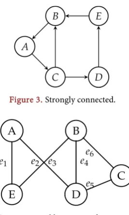
The digraph in Figure 3 is strongly connected because there is a path between any two ordered vertices in the directed graph. The digraph in Figure 4 is not strongly connected, since, for example, there is no directed path from S to T, nor from V to T, but it is weakly connected.

4. Matrices in Graphs

(6)

[image:6.595.146.543.46.763.2]

DOI: 10.4236/ojdm.2018.84008 84 Open Journal of Discrete Mathematics Figure 3. Strongly connected.

Figure 4. Weakly connected.

4.1. Matrices for Undirected Graph

Given an undirected graph G with n vertices and m edges. The adjacency matrix

of G V E

(

,

)

is given by A=

{ }

a_{ij n n}_× , where

1 if node is adjacent to node 0 otherwise

i j

ij

v v

a =  

The incidence matrix is given by M=

{ }

m_{i j n m}, _× , where

1 when edge is incident with node

0 otherwise j i

ij

e v

m =  

The Laplacian matrix can be found by using the relation

,

= −

L D A

where D is a diagonal matrix whose ith diagonal entry is the degree of the ith node and A is the adjacency matrix.

In other words, L=

{ }

l_{ij n n}_× , where

( )

1 if node is adjacent to node

if

0 otherwise

i j

ij i

v v

l deg v i j

−  

=_ =

 

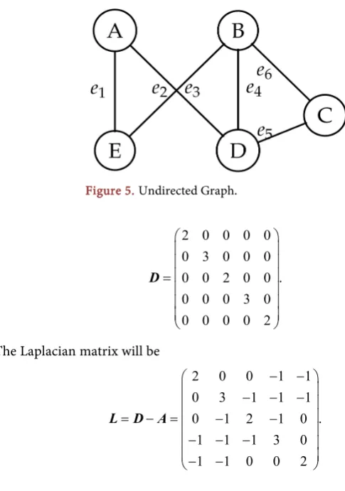
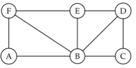
Figure 5 is undirected graph with five nodes and six edges where there is a path from one node to the other nodes. The adjacency matrix A, the incidence matrix M and the diagonal matrix D will be

0 0 0 1 1 1 1 0 0 0 0

0 0 1 1 1 0 0 1 1 0 1

, ,

0 1 0 1 0 0 0 0 0 1 1

1 1 1 0 0 0 1 0 1 1 0

1 1 0 0 0 1 0 1 0 0 0

   

   

= =

   

   

[image:6.595.306.440.65.288.2]

(7)

[image:7.595.221.464.65.411.2]

DOI: 10.4236/ojdm.2018.84008 85 Open Journal of Discrete Mathematics Figure 5. Undirected Graph.

2 0 0 0 0 0 3 0 0 0 . 0 0 2 0 0 0 0 0 3 0 0 0 0 0 2

 

 

=

 

 

D

The Laplacian matrix will be

2 0 0 1 1

0 3 1 1 1

.

0 1 2 1 0

1 1 1 3 0

1 1 0 0 2

− −

 

 ₋ ₋ ₋ 

 

= − = − −

 

− − −

 

₋ ₋ 

 

L D A

4.2. Matrices for Directed Graph

Given a directed graph G with n nodes and m edges. The adjacency matrix of

(

,

)

G V E is given by A=

{ }

a_{ij n n}_× , where

1 if node is connected to node and directed from to

0 otherwise

i j i j

ij i j j i

v v v v

a v v v v

  = −

 

The incidence matrix is given by M=

{ }

m_{i j n m}, _× , where

1 if node is the starting node of an edge

1 if node is the end node of an edge

0 otherwise

i j

ij i j

v e

m v e

  = −_

 

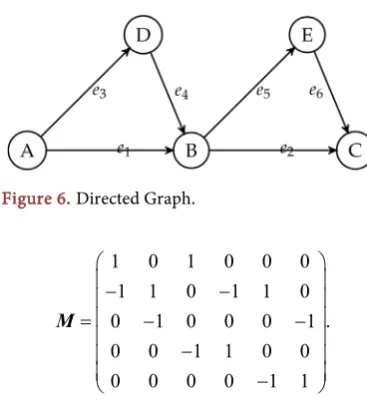
Figure 6 is a digraph which shows that there is path from node A to any other node of the graph, nevertheless there is no path from node C to any other node of the network. The adjacency matrix A and the incidence matrix M will be

0 1 0 1 0

1 0 1 1 1

,

0 1 0 0 1

1 1 0 0 0

0 1 1 0 0

 

₋ ₋ 

 

= − −

 

−

 

 ₋ 

 

(8)

[image:8.595.276.460.66.271.2]

DOI: 10.4236/ojdm.2018.84008 86 Open Journal of Discrete Mathematics Figure 6. Directed Graph.

1 0 1 0 0 0

1 1 0 1 1 0

.

0 1 0 0 0 1

0 0 1 1 0 0

0 0 0 0 1 1

 

₋ ₋ 

 

= − −

 

−

 

 ₋ 

 

M

4.3. Distance in Graphs

Geodesic distance denoted as d v v

(

0.

d D C = d A E = d D D =

The distance matrix of a graph, denoted as D, is the square matrix

{

d ij

( )

}

_{n n}_× , where d ij

( )

is equal to the length of the shortest path from node vi to node

j

v .

Consider the undirected unweighted graph in Figure 7 as example; The distance matrix for the graph in Figure 7, is given as;

0 1 2 2 2 1 1 0 1 1 1 1 2 1 0 1 2 2

. 2 1 1 0 1 2 2 1 2 1 0 1 1 1 2 2 1 0

 

 

=  

 

 

D

4.4. Perron—Frobenius Theorem

We will state (without giving the proof) the Perron-Frobenius theorem which will be used later on in our work.

Theorem 1 (Perron-Frobenius theorem). Let _A_∈_n n×

be an irreducible matrix. Then the Perron-Frobenius theorem states that [12]:

• A has a principal eigenvalue λ1 such that all other eigenvalues λi, for 2,3, ,

i= _ n_,_satisfy

(9)

[image:9.595.305.445.69.139.2]

DOI: 10.4236/ojdm.2018.84008 87 Open Journal of Discrete Mathematics Figure 7. Unweighted-Undirected Graph.

• _{The principal eigenvalue}λ₁_{has algebraic and geometry multiplicity of 1, and}

has a right eigenvector x with all positive elements, i.e. xi > ∀ =0, i 1,2, , n

and a left eigenvector v with all positive elements, i.e. vi= ∀ =0, i 1,2, , n. • _{Any non-negative right eigenvector is a multiple of} x, any non-negative left

eigenvector is a multiple of v.

Furthermore, if A is the adjacency matrix of a directed network with a strongly connected component, then

• A has a principal eigenvalue λ1 such that all other eigenvalues λi, for 2,3, ,

i=  n, satisfy

1 i .

λ ≥ λ

• _{The principal eigenvalue}λ₁ has algebraic and geometric multiplicity equal to 1, and has a left eigenvector x with non-negative elements, i.e. xi >0 if

node i belongs to the strongly connected component of the network or the out-components of the network, and xi =0 if node i belongs to the

in-component of the strongly connected component of the network.

5. Centrality Measures

Centrality of a given node is a measure of the importance and influence of that node in the corresponding network. The identification of which nodes are more important or central than the others is a key issue in network analysis. We can ask the following questions:

• _{Which are the most central nodes in a network?} • _{Which are the most important nodes in a network?} • _{Which are the most influential nodes in a network?}

These types of questions can have different interpretations in different networks. For instance;

• _{when dealing with a social network, the most central node can be the most}

popular person,

• _{when dealing with a web portal network, the most central node can be a web}

page with the best quality of content in a specific field,

• _{in terms of the internet network, the most central node might be a network}

gateway (router) with the highest bandwidth.

These ideas can be used to characterize types of centrality measure to find the most important nodes in a network in a given context. That is, there are many different centrality measures. When measuring the centrality of the node, we should be sure that:

(10)

DOI: 10.4236/ojdm.2018.84008 88 Open Journal of Discrete Mathematics • _{what they measure well; and}

• _{why a particular centrality measure is the most appropriate for the kind of set}

we are investigating.

The most common centrality measures include degree centrality, betweenness centrality, eigenvector centrality, Katz centrality, PageRank centrality, closeness centrality and subgraph centrality [11] [13].

5.1. Degree Centrality

Degree centrality of a node vi in a given network is given by the total degree i

d of vi. The degree centrality measures the ability of a node to communicate

directly with other nodes.

In an undirected network, the degree di of a node is given as

T

1 ,

n

i ij i

j

d a

=

∑

=e Ae (1)

where A is the adjacency matrix, ei is the ith standard basis vector (ith

column of the identity matrix) and e is the vector of all entries one. In a directed network, we can consider the in-degree of a node, given as

T

1 ,

n in

i ij i

j

d a

=

∑

=e Ae (2)

or the out-degree of the node, given as

T

1 .

n out

i ij i

j

d a

=

∑

=e Ae (3)

In a directed graph, a source is a node with zero in-degree and a sink is a node with zero out-degree.

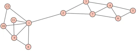
As an example, consider the undirected graph in Figure 8. We are interested in finding the central node using degree centrality.

The adjacency matrix A for Network-1 in Figure 8 is given as

0 1 0 0 0 0 0 1 1 1 1 1 1 0 1 0 0 0 1 0 0 0 0 0 0 1 0 1 0 0 1 0 0 0 0 0 0 0 1 0 1 1 1 0 0 0 0 0 0 0 0 1 0 1 0 0 0 0 0 0 0 0 0 1 1 0 1 0 0 0 0 0 0 1 1 1 0 1 0 0 0 0 0 0 1 0 0 0 0 0 0 0 1 0 0 0 1 0 0 0 0 0 0 1 0 1 1 0 1 0 0 0 0 0 0 0 1 0 0 1 1 0 0 0 0 0 0 0 1 0 0 0 1 0 0 0 0 0 0 0 0 1 0 0

 

 

=  

 

 

A

The degree centralities are contained in the vector d Ae= ;

[

]

T

(11)

[image:11.595.242.512.76.180.2]

DOI: 10.4236/ojdm.2018.84008 89 Open Journal of Discrete Mathematics Figure 8. Network-1.

Using the degree centrality measure, node 1 is the most central node due to the fact that it has the highest degree.

5.2. Closeness Centrality

 

 

D

(12)

T T

,

1 1

i i

i d

l

N N

= =

− −

e De e

where De=d

[

20 20 24 29 38 30 23 29 27 28 29 29

]

=

EVC

Thus, i 1 i c

l

= _{, gives}

1 11₂₀ 0.55, 2 11₂₀ 0.55, 3 11₂₄ 0.458

c = = c = = c = =

4 11₂₉ 0.379, 5 11₃₈ 0.289, 6 11₃₀ 0.367

c = = c = = c = =

7 11₂₃ 0.478, 8 11₂₉ 0.379, 9 11₂₇ 0.407

c = = c = = c = =

10 11₂₈ 0.393, 11 11₂₉ 0.379, 12 11₂₉ 0.379.

c = = c = = c = =

Now, nodes 1 and 2 are identified as the most important nodes in the network.

5.3. Eigenvector Centrality

In an undirected network which is connected we can write the measure of centrality by using the eigenvector centrality. Eigenvector centrality takes into consideration the importance of neighbours of a node. In degree centrality a node is awarded one centrality point for each neighbour. Eigenvector centrality gives each node a score which is proportional to the sum of the score of its neighbours. In eigenvector centrality, a node is important if it is linked to other important nodes. The larger an entry on the node, the more important the node is considered to be.

From the Perron-Frobenius theorem, the eigenvector associated to the principal eigenvalue of the adjacency matrix A is unique if the network is strongly connected. We define the centrality of a node iteratively by using the sum of its neighbours’ centralities. We initially assume that a node j has centrality ( )0 ₁

j

x = . Then we calculate a new iteration ( )1

i

x as the sum of the centralities of i’s neighbours.

That is,

( )1 ( )0_,

i ij j j

x =

∑

a x ₍₆₎

where aij are the entries of the adjacency matrix.

In matrix form we write this as:

( )1 ₌ ( )0_.

x Ax (7) After k-steps, we have

( )k ₌ ( ) ( )k 0_.

x A x (8) Note that the eigenvector centrality is defined as lim ( )k

k→∞ x .

We can write _x( )0 _{as a linear combination of eigenvectors}

i

(13)

adjacency matrix A, that is,

( )0 _,

i i

i c v

=

∑

x (9)

where the ci are constants.

Then, from Equation (8), we have

( ) ( ) ( )

1 1

.

k k

k k k k k i k i

i i i i i i i i i i i

i c v i c v i c v i c v i c v

λ λ

λ λ λ

λ λ

   

= = = = _{ } = _{ }

   

∑

x A A (10)

Therefore, ( ) 1 1 , k k i i i k

i c v

λ λ λ   = _{ }  

∑

x ₍₁₁₎

where λi is the eigenvalue associated with the eigenvector vi and λ1 is the

principal eigenvalue. Since 1 1 i λ

λ < , for i=2,3, , n, we have;

1 1

1

lim lim lim

k k

k

i i

i i i i

k

k k _i c v _i c k v c v

λ λ λ λ λ →∞ →∞ →∞     = _{ } = _{ } =    

∑

x as 1

lim 0, 1.

k i k i λ λ →∞  

→ ∀ >  

 

This implies that the limiting centralities are proportional to the principal eigenvector v1 of the adjacency matrix.

Therefore, in matrix form, the eigenvector centrality x satisfies

1 1 1 λ λ = ⇒ =

Ax x x Ax (12)

1

1 _.

i ij j

j

x =_λ

∑

a x ₍₁₃₎

Note that in eigenvector centrality, the higher the centrality of the neighbours of the node, the more important the node is.

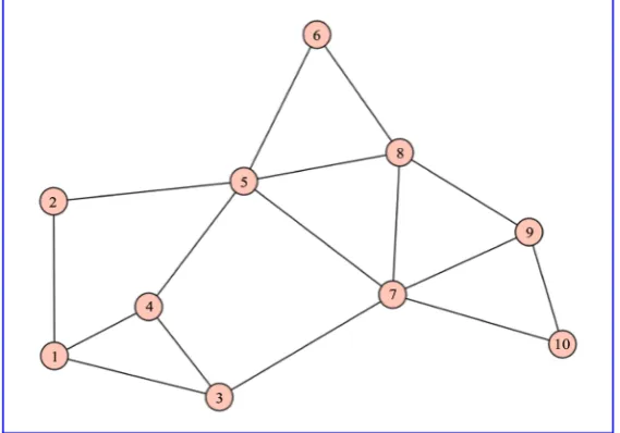
For example, consider the network in Figure 9.

The adjacency matrix for Network-2 in Figure 9, is given by

0 1 1 1 0 0 0 0 0 0 1 0 0 0 1 0 0 0 0 0 1 0 0 1 0 0 1 0 0 0 1 0 1 0 1 0 0 0 0 0 0 1 0 1 0 1 1 1 0 0

. 0 0 0 0 1 0 0 1 0 0 0 0 1 0 1 0 0 1 1 1 0 0 0 0 1 1 1 0 1 0 0 0 0 0 0 0 1 1 0 1 0 0 0 0 0 0 1 0 1 0

(14)

[image:14.595.232.517.74.273.2]

DOI: 10.4236/ojdm.2018.84008 92 Open Journal of Discrete Mathematics Figure 9. Network-2.

The eigenvalues of the adjacency matrix are

( ) (

)

2.464, 1.931, 1.543, 0.666, 0.477, 0.332,0.370,1.398,2.116,3.531 A

ρ

= − − − − −

−

The principal eigenvector corresponding to the principal eigenvalue

1 3.531

λ = _is

[

]

0.198 0.181 0.261 0.255 0.443 0.243 0.468 0.416 0.313 0.221 v=

Since the eigenvector centralities ( EVC ) correspond to the principal eigenvector, the eigenvector centralities for Network-2 will be

[

]

0.198 0.181 0.261 0.255 0.443 0.243 0.468 0.416 0.313 0.221

=

EVC

Using the eigenvector centrality, we conclude that node 7 is the most important node.

5.4. Katz Centrality

Katz centrality takes into consideration both the number of direct neighbours and the further connections of a node in the network. That is, a node is important in Katz centrality if it has universal connections to other nodes in the network. Katz centrality takes into account all paths of arbitrary length from a node i to other nodes in the network.

The Katz centrality k is given by

( )

0 0 ,

k k k

k k

α α

∞ ∞

= =

 

=_ _ =



∑



∑

k A e A e (14) where e is the column vector of ones, α is called the attenuation factor and

(15)

( )

(

( )

2

)

0 ,

k k

α α α

∞

=

∑

= + + +

k A e I A A  e (15) and, if the sum converges, then

(

)

1

,

α −

= −

k I A e (16)

where I is n n× _{identity matrix and} e is the column vector of ones. To ensure the convergence of

(

α

)

−1

−

I A and an accurate definition of Katz centrality, we must consider the attenuation factor α _{to be within the range}

1

1 0,

α

λ

 

∈ 

 .

For example, we compute the Katz centrality of Network-2 in Figure 9. Since the principal eigenvalue is λ =1 3.531, then α∈0,_3.5311 

 . To calculate the

Katz centrality, we choose

α

=0.25_{, then the Katz centrality will be}

(

_0.25

)

−1 _,

= −

k I A e

[

]

T

5.826 5.223 7.086 6.992 11.065 6.316 11.526 10.201 7.895 5.855

⇒ =k

Therefore, node 7 is the most important node.

5.5. Subgraph Centrality

Subgraph centrality attempts to measures the centrality of a node by taking into consideration the participation of each node in all subgraphs of the network. It does this indirectly by counting the number of closed walks in the network which start and end at a given node in the network: a relationship can be shown between subgraphs and these walks.

If A is the adjacency matrix of an unweighted network, we know that

•

2 3

0 ! 0 ! 1! 2! 3!

k

k ii

k k _ii

i SC i

k k

µ

∞ ∞

= =

 

= = =_ + + + + _

 

∑

A I A A A  (17)

( )

e _ii SC i

(16)

Considering the exponential of the adjacency matrix,

2 3

e

2! 3! !

k

= + + + + + +

A _{I A} A A _ A _

we observe that the numbers of closed walks associated with _A2_{of length 2 are}

counted twice for every link in the network. On the other hand, the closed walk associated with _A3_{of length 3 is counted} _{2 3 3!}_{× =} _{for every triangle. To}

avoid double counting, we penalize the closed walks of length 2 by 2! and closed walks of length 3 are penalized by 3!. In general, any circuit of length k

can be traversed in 2 directions and there are k points where you can start, so that this circuit is counted 2×k_{times. From the exponential of the adjacency} matrix, when k≥4 _{, the penalization included is not the same as the}

penalization of counting the number of repeated closed walks.

For instance, let us consider Network-2 in Figure 9. We want to find the subgraph centrality. We have;

3.962 2.475 3.393 3.532 2.914 0.991 2.345 1.569 0.944 0.687 2.475 2.79 1.858 2.227 3.306 1.423 2.188 1.997 1.055 0.682 3.393 1.858 4.283 3.696 3.498 1.369 4.021 2.631 2.037 1.562 3.532 2.227 3.696 4.345 4.107 1.691 3.297 2.564 1.508 1.0

eA=

44 2.914 3.306 3.498 4.107 7.713 4.312 6.554 6.404 3.924 2.556 0.991 1.423 1.369 1.691 4.312 3.423 3.448 4.131 2.24 1.294 2.345 2.188 4.021 3.297 6.554 3.448 8.37 6.791 5.762 4.327 1.569 1.997 2.631 2.564 6.404 4.131 6.791 7.02 4.948 3.131 0

.

.944 1.055 2.037 1.508 3.924 2.24 5.762 4.948 5.016 3.563 0.687 0.682 1.562 1.044 2.556 1.294 4.327 3.131 3.563 3.32

 

 

 

Then the subgraph centrality will consist of the diagonal entries of eA_{, which}

is

( )

[

]

T

3.962 2.79 4.283 4.345 7.713 3.423 8.37 7.02 5.016 3.32 SC i =

We observe that node 7 has the highest subgraph centrality, thus, node 7 is the most central node.

6. Relationship between Centrality Measures

(17)

1

0 and .

α α

λ

→ →

We will prove these correlations and stability of ranking. This will relate the degree and eigenvector centrality to Katz centrality.

Theorem 2. Let G=

(

V E,

)

_{be undirected connected network with}

adjacency matrix A. The Katz centrality k is given as

(

)

1

.

α −

= −

k I A e

Then,

• _as

α

→0_{, the ranking produced by}k converges to that produced by degree centrality, and

• _as

1

α λ

→ _{, the ranking produced by}k converges to that produced by

eigenvector centrality.

Proof. The Katz centrality k is given as

(

_α

)

−1 _,

= −

k I A e (19)

which can be written as

(

)

( ) ( )

(

)

( )

1

2 3

α

α α α

−

= −

= + + + +

k I A e

I A A A e

e Ae A e A e



(20)

( )

2

( )

3

α α α

= + + + +

k e d A e A e  (21)

where d is the vector of the degree centralities of the nodes. Consider the relation

(

)

1 _.

ψ α

= k e− (22) It is clear that the ranking produced by

ψ

_{will be exactly the same as that}

produced by k, due to the fact that the score of each node has been scaled and shifted in the same way. Thus,

(

)

(

( )

2

( )

3

)

1 1

ψ α α α

α α

= k e− = e+ d+ A e+ A e+

2 2 3 _.

ψ = +d αA e+α A e+ (23) Then,

0

lim

α→ψ =d (24)

where d is the vector of the degree centralities of the nodes.

Therefore, the ranking produced by the Katz centrality reduces to that produced by degree centrality.

To show the second relation, we write the column vector e, as

1 ,

n i i i= β

=

∑

(18)

where β′is are constants and vi′s are eigenvectors of matrix A.

Then, we can write the Katz centrality as

(

)

( )

1

0

0 1 0 1

0 1 1

1 1

k

n n

k k k

i i i i

k i k i

n n

k k

i i i i i

k i i i

α α

α β α β

α β λ β

αλ ∞ − = ∞ ∞ = = = = ∞ = = = = − = = = = = −

∑

∑ ∑

∑

k I A e A e

A v A v

v v (26) 1 1 =2 1 1 1 1 2 1 1 1 1 1 1 1 1 1 n i i i i n i i i i β β αλ αλ αλ β β

αλ = αλ

⇒ = + − −  −  =  +  − _ − _

∑

k v v

v v

(27)

Consider the relation

(

1 1

)

φ= −αλ k (28) That is, the ranking produced by

φ

_{is exactly the same as that produced by}

k, due to the fact that the score of each node has been scaled and shifted in the same way. This implies that

1 1 1 2 1 = 1 n i i i i αλ

φ β β

αλ = − + −

∑

v v (29)

Then, 1 1 1 1 lim α λ

φ β

→

= v (30)

This implies that the limiting centralities are proportional to the principal eigenvector v1 of the adjacency matrix. Thus, the ranking produced by the Katz

centrality reduces to those produced by eigenvector centrality.

7. Matrix Functions

This section discusses some of the matrix functions developed using Taylor series.

Matrix functions have applications throughout applied mathematics and scientific computing. Matrix functions are used in various fields, for example, in control theory and electromagnetism and can also be used to study complex networks like social networks.

f z =a a z a z+ + +_ ₍₃₁₎

for z R< , and a kk, ≥0 are complex-valued constants [12].

Let _A_∈_Cn n× _{be a complex-valued matrix. Then we define the matrix}

(19)

( )

2

0 1 2 .

f A =a I+a A+a A + (32)

The matrix series in Equation (32) is convergent to the n n× _matrix f

( )

A

∑

(33)

in an open disc z R< . Then the series

0 k k k a ∞ =

∑

A (34)

is convergent if and only if the eigenvalues of A lie in z R< _[12]_.

Proof. We prove this theorem only for diagonalisable matrices using the Jordan form of matrix A.

Let Q be a transformation matrix which diagonalizes A. Then we can write

(

)

1

1, , n .

diag

λ

−

= =

D  Q AQ (35)

Thus,

( )

(

( )

)

(

)

1 1 1 1 0 0 1 0 1 0 0 , , , , . n k k

k k n

k k k k k k k k k k k

f diag f f

diag a a

a a a λ λ λ λ − ∞ ∞ − = = ∞ − = ∞ − = ∞ = =   = _ _     = _ _ = =

∑

A Q Q

Q Q

Q D Q

QDQ

A



(36)

If A has an eigenvalue λi ≥R, then the series in Equation (33) diverges

when evaluated at λi. It follows that the series in Equation (34) also diverges.

That is, if there exist eigenvalues of matrix A which fall outside z R< , then the series in Equation (34) diverges.

Therefore f

( )

A converges if and only if λi <R, where λ ≤ ≤i,1 i n are the

eigenvalues of matrix A.

In general, if the function f z

( )

can be expressed by using Taylor series and it converges in the disc z R< _{which contains the eigenvalues of}A, then

( )

f A can be computed by substituting the matrix A for variable z in the function f z

( )

. For instance,

( )

1

( ) (

) (

1

)

1

z

f z f

z

− +

= ⇒ = − +

− A I A I A

(20)

DOI: 10.4236/ojdm.2018.84008 98 Open Journal of Discrete Mathematics • _{Exponential function}

( )

2 3

0

e 1

2! 3! !

k z

k

z z z

f z z

k

∞

=

= = + + + +=

∑

(37)

k

z z z

f z z

k

∞

= −

= = − + +=

∑

( )

cos

( )

2 4

2! 4! f

⇒ A = A = −I A +A +

( )

_{( )}

2

0 1 cos 2 ! k k k k ∞ = −

=

∑

A

A (39)

• _{Sine function}

( )

3 5

( )

₍

2 1

₎

0

1 sin

3! 5! 2 1 !

k k

k

z z z

f z z z

k + ∞ = − = = − + + = +

∑



( )

3 5

( )

₍

2 1

₎

0

1

sin .

3! 5! 2 1 !

k k k f k + ∞ = − ⇒ = = − + + = +

∑

A A A

A A A  (40)

• _{Logarithmic function}

( )

(

)

2 3 4

( )

( 1)

1

1 log 1

2 3 4

k k

k

z z z z

f z z z

k

+ ∞

= −

= + = − + − +=

∑

(41)

( )

(

)

2 3 4

( )

( 1)

1

log .

2 3 4

k k k f k + ∞ = −

⇒ A = I A+ = −A A +A −A +=

∑

A (42)

• _{Hyperbolic function}

1) sinh function

( )

3 5

₍

2 1

₎

0

sinh

3! 5! 2 1 !

k k

z z z

f z z z

k + ∞ = = = + + + = +

∑



( )

3 5

₍

2 1

₎

0

sinh

3! 5! 2 1 !

k k f k + ∞ = ⇒ = = + + + = +

∑

A A A

A A A 

2) cosh function

( )

2 4

_{( )}

2

0

cosh 1

2! 4! 2 !

k k

z z z

f z z

k ∞

=

= = + + +=

∑

( )

2 4

_{( )}

2

0

cosh .

2! 4! 2 !

k k f k ∞ =

⇒ A = A = +I A +A +=

∑

A

(21)

of all the nodes we can compute f

( )

A e, where e is the vector of ones, or

( )

(

)

diag f A .

We may need to be careful with these raw centrality measures as f

( )

A may contain negative (or even complex) entries. For instance, to compute the logarithmic function f

( )

A , we need to take care of the complex entries, since it is not possible to make ranking out of complex entries. To avoid the complex entries, we compute log

(

γI A+

)

, where

γ

is a real constant chosen so that

(

γI A+

)

has positive eigenvalues. The constant

γ

_{differs for different}

networks.

We can also define centrality measures by applying analytic continuations of

( )

f z outside its radius of convergence. Recall that, if the attenuation factor

1

α λ

< _{, where}λ₁_{is the principal}

eigenvalue of A, then

(

)

1

0 .

k k

k I

α α

∞ ₋

=

= −

∑

A A

But

( ) (

)

1

f I α −

= −

A A

is also defined for

1

α λ

≥ _{as long as} 1

i

α λ

≠ _where λ_i is an eigenvalue of

A. Then we can generalize Katz centrality by the following definition:

(

)

1

(

)

1

_{( )}

1

diag I α or I α withα

ρ

− −

= − = − >

k A k A e

A

where e is the column vector of ones and ρ

( )

A is the spectrum of A. To determine which of the matrix functions can be used to asses centrality in the network, we will do some experimental work on a variety of networks in the following section. We will perform the experimental work by making comparisons between the rankings based on the common centrality measures discussed in section V and the rankings based on these matrix functions.

8. Experimental Work and Discussion

In this section we aim to analyse experimentally the agreements between the centrality measures discussed in section V, and whether the matrix functions discussed in section VII can be used to determine the important nodes in a network. The experimental work will compare matrix functions to the common centrality measures.

A variety of techniques can be used to compute centrality measures (those discussed in section V) and matrix functions. To compute the exponential of a matrix, logarithmic of a matrix and other matrix functions we will use SciPy

(22)

coefficient in our experiments to compare the agreement between centrality measures.

8.1. Correlation (Kendall, Pearson, Spearman) Coefficient

Correlation is a bivariate analysis that measures the strengths of association between two variables. The value of the correlation coefficient varies between 1 and −1. The positive correlation signifies that the ranks of both variables are increasing, while the negative correlation signifies that as the rank of one variable increases, the rank of the other variable is decreasing. The correlation coefficient between the two variables is said to be a perfect association if it lies between ±1 [15]. The closer the value of the correlation coefficient to 1 or to −1, the stronger the relationship between the two variables. As the correlation coefficient value goes towards 0, the relationship between the two variables will be weaker. In statistics, we usually measure the strengths of association by: Pearson correlation, Kendall rank correlation and Spearman correlation.

The Kendall coefficient of correlation is the measure of the degree of correspondence between two set of ranks given to the same set of objects. The Kendall coefficient is interpreted as the difference between the probability of these objects being in the same order and the probability of these objects being in a different order [2].

Let X and Y be two observations, such that

(

x y1, 1

) (

, x y2, 2

and

(

x yj, j

)

is said to be concordant if

0,

i j i j

x x

y y

− > −

which implies that either x xi> j and yi>yj or x xi< j and yi<yj.

• _{The pair is said to be}_discordant_if 0,

i j i j

x x

y y

− < −

which implies that either x xi> j and yi<yj or x xi< j and yi>yj.

• _{The pair is neither}_concordant_nor_discordant_if x x_i= _j_or y_i =y_j_.

The Kendall

( )

τ _{correlation coefficient} is defined as

(

)

o o

N concordant pairs N discordant pairs

1 ₁

2n n

τ= −

−

The Kendall rank coefficient can be interpreted as follows: the values of τ

greater than zero show an agreement, being close to one indicates a strong agreement. On the other hand, values less than zero show a disagreement and those close to negative one indicate a strong disagreement [2]. Indeed, if all pairs are concordant, then

τ

=1_{, which implies that the variables are in exactly the}

(23)

the variables are in exactly the opposite ranking (order).

Pearson correlation is a measure of degree of linear relationship between two variables and is denoted by r. Pearson correlation is basically used to draw a line of best fit through the data of two variables, r indicates how far away all these data points are to the line of best fit.

The following formula is used to calculate the Pearson r correlation:

( )

(

₂ 2

)

(

₂

( )

2

)

N xy x y r

N x x N y y

− =

− −

∑

∑ ∑

∑

(43)

where:

r = Pearson correlation coefficient

N = number of observation in each data set

xy

∑

= the sum of the products of paired scores

x

= sum of squared scores of variable y

To use Pearson correlation r, the two variables must be measured either in interval or ratio scale. However, both variables do not need to be measured on the same scale (for instance, one variable can be ratio and one can be interval). We can not use the Pearson correlation for ordinal data, instead we use Spearman’s rank correlation or a Kendall’s Correlation.

Spearman rank correlation is the nonparametric version of the Pearson correlation coefficient that is used to measure the degree of association between two two continuous or ordinal variables.

The following formula is used to calculate the Spearman rank correlation:

(

)

2

6 1

1 i D N N

ρ = −

−

∑

₍₄₄₎

where; D Ri= x_i −Ry_i is the difference between the two ranks of each

observation; N is the number of observations.

We use the Spearman correlation coefficient when the relationship between variables is not linear.

Despite the fact that both Spearman and Kendall correlations measure monotonicity relationships and have a nice interpretation but in this paper we will opt to use the Kendall correlation coefficient due to the following reasons [16] [17]:

• _{The distribution of Kendall’s has better statistical properties.}

• _{The interpretation of Kendall’s in terms of the probabilities of observing the}

agreeable (concordant) and non-agreeable (discordant) pairs is very direct.

• _{The Kendall correlation has a smaller gross error sensitivity (GES) (more}

(24)

(

log

)

O n n of Spearman correlation, where n is the sample size.

8.2. Network Models

Networks have been around us for so many years and the study is not new. Graph theorists and mathematicians have been surrounded by problems where they were trying to make sense of these complex networks. As a result of this, random network theory was generated stating that nodes and links in a graph are connected randomly to each other. In this paper we will consider three networks model due to its significance:

• _{Erdös-Rényi model: are formed by completely random interactions between}

the nodes. Each node chooses its neighbours at random, constrained either by an overall number of relationships that might be assigned in the graph, or a probability of connecting to a certain neighbour [18]. Mathematically, each network would be following a poison distribution. This distribution is such that vast majority of nodes have equal number of links and it is almost impossible to find outliers.

• _{Barabási-Albert model: these are scale-free networks which are formed by}

two simple mechanisms, growth and preferential attachment. The main prediction which a scale free network makes is the presence of few outlier nodes which have many connections. These nodes are also known as hubs. Preferential attachment is a probabilistic mechanism in which a new node is free to connect to any node in the network, whether it is a hub or has a single link [18] [19].

• _{Watts-Strogatz model: is important because it shows how the “small-world}

effect” in networks can coexist with other commonly observed features of social networks, like a high clustering coefficient. More specifically, the model showed how adding a small fraction of random long-range links in an otherwise regular network can lead to slow, logarithmic scaling of the typical distance between nodes with network size [20].

8.2.1. First Experiment

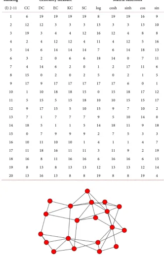
We begin our experiments by considering a small network with 20 nodes. The network was randomly generated in text editor and drawn using Sage. The aim is to determine which of the matrix functions give similar rankings as the common centrality measures. We have many functions to choose from and we want to limit our choice. Note that we will not consider the exponential functions since it is similar to the subgraph centrality.

The experiment shows that the diagonal entries of the logarithmic function and cosine function give the ranking of the nodes in reverse order as compared to other rankings. Also, we observe that the sine function does not match any other centrality measure. The network in Figure 10, having 20 nodes and 42 edges gives us a real picture on node ranking.

(25)

[image:25.595.208.538.102.632.2]

DOI: 10.4236/ojdm.2018.84008 103 Open Journal of Discrete Mathematics Table 1. Rankings of nodes using centrality measures and matrix functions for the net-work in Figure 10.

Ranking Centrality measure Matrix functions

(l) 2-11 CC DC EC KC SC log cosh sinh cos sin

1 6 19 19 19 19 8 19 19 16 9

2 12 12 3 3 3 13 3 3 13 10

3 19 3 4 4 12 16 12 4 8 8

4 2 4 12 12 4 11 4 12 5 16

5 14 6 14 14 14 7 6 14 18 13

6 3 2 0 6 6 18 14 0 7 11

7 4 14 6 2 0 1 2 17 11 6

8 15 0 2 0 2 5 0 2 1 5

9 17 9 17 17 17 17 17 6 0 1

10 1 10 18 18 15 0 15 18 17 12

11 5 15 5 15 18 10 10 15 15 17

12 9 17 15 5 10 15 9 7 10 2

13 7 1 7 7 7 9 5 10 14 0

14 18 5 1 1 5 14 18 11 9 18

15 0 7 9 9 9 2 7 5 3 3

16 10 11 10 10 1 4 1 1 4 7

17 11 18 16 11 11 3 11 9 2 19

18 16 8 11 16 16 6 16 16 6 15

19 8 13 8 13 13 12 13 13 12 14

[image:25.595.206.539.111.634.2]

20 13 16 13 8 8 19 8 8 19 4

Figure 10. Network with 20 nodes and 42 edges.

Note that the ranking is from the most to the least important/central node with respect to the centrality measure used.

(26)

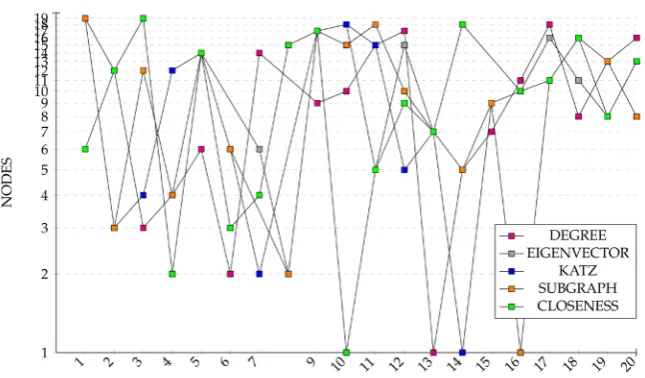
functions, we will choose one centrality measure among the other one. To do this we need to investigate whether the chosen centrality measure agrees with the other centralities measures. In this case, we make a comparison between the closeness centrality (CC) and degree centrality (DC), eigenvector centrality (EC), Katz centrality (KC) and subgraph centrality (SC) for graph in Figure 10.

Table 2 shows that there is an agreement between closeness centrality and other centrality measures.

We observe from graph of Figure 11 that there is an agreement between closeness centrality and other centrality measures.

In Table 1, we have to modify the cosine and logarithmic functions so that they match with other rankings. The best way of doing this seems to be by reversing the order of their rankings.

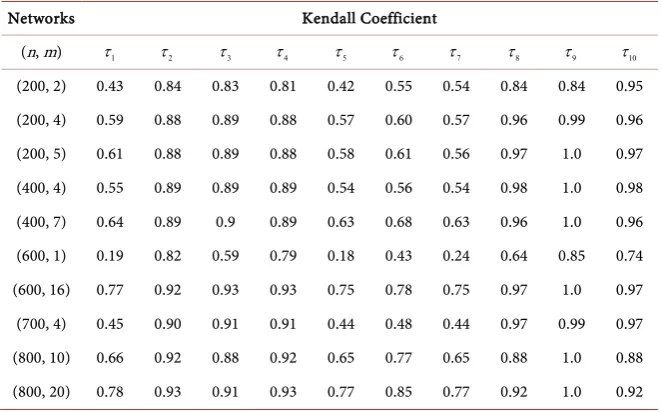
To be more confident about the rankings of nodes using matrix functions, we will use the Kendall correlation coefficient to make the comparison between closeness centrality and the matrix functions. We chose closeness centrality among the other standard centrality measure to make the comparison with matrix functions in as much as it takes into account neighbours and the neighbours of neighbours of a node to determine its centrality. In the comparisons, we denote by τ