Second Kind Shifted Chebyshev Polynomials for Solving the Model Nonlinear ODEs

(1)

http://www.scirp.org/journal/ajcm ISSN Online: 2161-1211 ISSN Print: 2161-1203

DOI: 10.4236/ajcm.2017.74028 Oct. 26, 2017 391 American Journal of Computational Mathematics

Second Kind Shifted Chebyshev Polynomials for

Solving the Model Nonlinear ODEs

Amr M. S. Mahdy1,2, N. A. H. Mukhtar3

1_{Department of Mathematics, Faculty of Science, Zagazig University, Zagazig, Egypt} 2_{Department of Mathematics, Faculty of Science, Taif University, Taif, KSA}

3_{Department of Mathematics, Faculty of Science, Benghazi University, Benghazi, Libya}

Abstract

In this paper, we build the integral collocation method by using the second shifted Chebyshev polynomials. The numerical method solving the model non-linear such as Riccati differential equation, Logistic differential equation and Multi-order ODEs. The properties of shifted Chebyshev polynomials of the second kind are presented. The finite difference method is used to solve this system of equations. Several numerical examples are provided to confirm the reliability and effectiveness of the proposed method.

Keywords

Chebyshev Spectral Method, Riccati Differential Equation, Logistic Differential Equation, Multi-Order ODEs

1. Introduction

In recent years, Chebyshev polynomials (family of orthogonal polynomials on the interval [−1, 1]) have become increasingly important in numerical analysis, from both theoretical and practical points of view. They have strong links with Fourier and Laurent series, with minimality properties in approximation theory and with discrete and continuous orthogonality in function spaces [1]. These links have led to important applications, especially in spectral methods for ordi-nary and partial differential equations. There are four kinds of Chebyshev poly-nomials as in [2]. The majority of books dealing with Chebyshev polynomials, contain mainly results of Chebyshev polynomials of all kinds Tn

( )

x U, n

( ) ( )

x V, n x

and Wn

( )

x and their numerous uses in different applications and research

pa-pers dealing with some types of these polynomials ([3]-[8]) and other publica-tions as ([9][10][11][12][13]). However, there are only a limited researches of literature on shifted Chebyshev polynomials of the second kind Un

( )

x

∗ _{, either}

How to cite this paper: Mahdy, A.M.S. and Mukhtar, N.A.H. (2017) Second Kind Shifted Chebyshev Polynomials for Solving the Model Nonlinear ODEs. American Journal of Computational Mathematics, 7, 391-401.

https://doi.org/10.4236/ajcm.2017.74028

Received: July 16, 2017 Accepted: October 23, 2017 Published: October 26, 2017

(2)

DOI: 10.4236/ajcm.2017.74028 392 American Journal of Computational Mathematics

from theoretical or practical points of view it uses in various applications.

2. Some Properties of Chebyshev Polynomials of the

Second Kind

2.1. Chebyshev Polynomials of the Second Kind ([2] [14])

The Chebyshev polynomials Un

( )

x of the second kind [2] are orthogonal

polynomials of degree n in x defined on the [−1, 1]

( )

sin

(

1

)

sin n

n

U x θ

θ

+ =

where x=cosθ and θ∈

[ ]

0,π . The polynomials Un

( )

x are orthogonal on

[

−1,1

]

with respect to the inner products

( )

(

)

1 ₂

( ) ( )

1

0,

, 1 d π

, 2

n m n m

n m

U x U x x U x U x x

n m

−

≠  

= − =  ₌



∫

(1)

where 2

1−x is weight function.

( )

n

U x may be generated by using the recurrence relations

( )

2 1

( )

2

( )

, 2, 3,

n n n

U x = xU ₋ x −U ₋ x n= 

with U0

( )

x =1, U1

( )

x =2x.

The analytical form of the Chebyshev polynomials of the second kind Un

( )

x

of degree n is given by:

( )

(

) (

)

π π

2

2 2

0 0

1

1 2 1 2 , 0.

1 2 1

n i

i n i i n i

n

i i

n i n i x

U x x n

i i n i

   

    −

  ₋  

−

= =

− Γ − +

 

= − _ _ = − >

Γ + Γ − +

 

∑

(2)

where π

2

   

  denotes the integral part of n 2.

2.2. Shifted Chebyshev Polynomials of the Second Kind ([2] [14])

In order to use these polynomials in Section 2.1 on the interval x∈

[ ]

0,1 we

define the so called shifted Chebyshev polynomials of the second kind Un

( )

x

∗

by introducing the change variable z=2x−1. This means that the shifted

Chebyshev polynomials of the second kind defined as ([2][14]):

( )

(

2 1

)

n n

U∗ x =U x−

also there are important relation between the shifted and second kind Chebyshev polynomials as follows:

( )

2

( )

1 2 1

2xUn x U n x ,

∗

− = −

these polynomials are orthogonal on the support interval

[ ]

0,1 as the following

inner product:

( )

(

)

1 ₂

( ) ( )

0

0, ,

, d _π

, ,

8

n m n m

n m

U x U x x x U x U x x

n m

∗ ∗ ∗ ∗

≠  

= − =  ₌



(3)

where 2

x−x is weight function.

( )

n

U∗ x may be generated by using the recurrence relations

( ) (

2 2 1

)

1

( )

2

( )

, 2,3,

n n n

U∗ x = x− U∗− x −U∗− x n= 

with start values U0

( )

x 1

∗ ₌

, U0

( )

x 4x 2

∗ ₌ ₋

.

The analytical form of the shifted Chebyshev polynomials of the second kind

( )

n

U∗ x of degree n is given by

( )

2 2

(

) (

)

0

2 2

1 2 , 0,

1 2 2 2

n i n

i n i n

i

n i x

U x n

i n i

−

∗ −

=

Γ − +

= − >

Γ + Γ − +

∑

(4)

The function which may be appear in solution of the model problem can be written as series of U∗

( )

x .

Let g x

( )

be a square integrable in

[ ]

0,1 it can be expressed in terms of the

shifted Chebyshev polynomials of the second kind as follows:

( )

0

,

i i i

g x a U x

∞ ∗

=

∑

(5)

where the coefficients a i_i, =0,1, are given by:

( )

1 ₂

1

2 1

1 d ,

π 2

i i

x

a = ₋ g_ + _ −x U x x

 

∫

(6)

or

( )

1 ₂ 0 8 d , i i

a g x x x U x x

π

∗

=

∫

− (7)

In practice, only the first

(

m+1

)

terms of shifted Chebyshev polynomials of

the second kind are considered in the approximate case. Then we have:

( )

0

, m

m i i

i

g x a U∗ x

=

∑

₍₈₎

Using the parctice shifted Chebyshev polynomials of the second kind to constraction the integral collocation method to give the N-th derivative of the unknown function u x

( )

as the following [15]:

( )

0 0

d

. d

k _m _m

k

n n n n

k

n n

u x

a U x a w x x

∗

= =

=

∑

 (9)

Using the integration we can obtain the lower-order derivatives and the function itself as follows

( )

1 1 1 1 0 d d k _m k n n n n u x

a w x c x − − − = +

∑

 (10)

( )

2 2 1 2 2 0 d , d k _m k n n n n u x

a w x c x c x − − − = + +

∑



 (11)

( )

(

)

(

)

2 3

1

1 2 2 1

0

d

,

d 2 ! 3 !

k k

m

n n k k

n

u x x x

a w x c c c x c

x k k

− − − − = + + + + + − −

∑



 (12)

( )

(

)

(

)

1 2

0

1 2 1

0

,

1 ! 2 !

k k

m

n n k k

n

x x

u x a w x c c c x c

k k − − − = = + + + + + − −

(4)

from (4) and (9) we have

( )

(

)

(

) (

)

2 2

0

2 2

1 2 ,

1 2 2 2

n i n

i

k n i

n i

n i x w x

i n i

− −

=

Γ − +

= −

Γ + Γ − +

∑

(14)

( )

(

)

(

) (

)(

)

1

1 2 2

0

2 2

d 1 2

1 2 2 2 1

n i n

i

k k n i

n n

i

n i x

w x w x x

i n i n i

− +

− −

=

Γ − +

= = −

Γ + Γ − + − +

∑

∫

,

( )

(

)

(

) (

)(

)

2

2 1 2 2

0

2 2

d 1 2

1 2 2 2 1 2

n i n

i

k k n i

n n

i

n i x

w x w x x

i n i n i n i

− +

− − −

=

Γ − +

= = −

Γ + Γ − + − + − +

∑

∫

,



( )

(

)

(

) (

)(

)

0 1 2 2

0

2 2

d 1 2

1 2 2 2 1

i k n

i n i

n n

i

n i x

w x w x x

i n i i k i k

+ −

=

Γ − +

= = −

Γ + Γ − + + − +

∑

∫

_ .

We now collocate Equatuions (10)-(14) at

(

m+1

)

points x_p,p=0,1,,m

as

( )

( ) 1

( )

( 1)

1

d d

ˆ_, ˆ_, _,

d d

k k

p k p k

k k

u x u x

E E

x x

−

− −

= Ω = Ω _ ₍₁₅₎

( )

( )1

( )

( )0

d

ˆ_, ˆ_,

d

p

u x

E u x E

x = Ω = Ω

where

[

]

T

0 1 1 2

ˆ _, _, _, _{, ,} _, _,

m n

E= a a  a c c  c , and Ω( )k ,Ω(k−1),,Ω( )0 are integrated

matrices.

3. Integral Collocation Method for Solving Riccati, Logistic

and Multi-Order Nonlinear ODEs [15]

In this section, we introduce the integral collocation method using shifted Chebyshev polynomials of the second kind for solving the Riccati, Logistic and multi-order nonlinear ODEs.

3.1. Model 1: Riccati Differential Equation [15]

( )

2

( )

d

1 0, 0,

d

u x

u x x

x + − = ≥ (16)

we also assume an initial condition

( )

0

.

u x =u (17)

The exact solution to this problem at 0

0

u = is

( )

22

e 1

.

e 1

x x

u x = −

+

The procedure of the implementation is given by the following steps:

1) Approximate the function u x

( )

using formula (9)-(14) with m=5, as

follows

( )

5 ( )

( )

1

0

d

,

d n n n

u x

a w x

(5)

( )

5 ( )

( )

0 1 0

, n n

n

u x a w x c

=

+

∑



where ( )0

( )

n

w x is defined in (14) as

( )

(

)

(

) (

)(

)

0 2 2

0

2 2

1 2

1 2 2 2 1

i k n

i n i n

i

n i x w x

i n i i k i k

+ −

=

Γ − +

= −

Γ + Γ − + + − +

∑

_

( )

(

)

(

) (

)

1 2 2

0

2 2

1 2 ,

1 2 2 2

n i n

i n i n

i

n i x w x

i n i

− −

=

Γ − +

= −

Γ + Γ − +

∑

Then the Riccati differential Equation (16) is transformed to the following approximated form

( )

2

5 5

0 1

0 0

1

n n n n

n n

a U∗ x a w x c

= =

 

+_ + _ =

 

∑

(19)

We now collocate Equation (19) at

(

m+ =1 6

)

points x_p,p=0,1, 2,3, 4,5

as

( )

2

5 5

0

1

0 0

1

n n p n n p

n n

a U∗ x a w x c

= =

 

+_ + _ =

 

∑

(20)

For suitable collocation points we use the roots of shifted Chebyshev polynomial U6

( )

x

∗ _.

2) Also, by substituting from the initial condition (17) in (18) we can obtain

(

n=1

)

an equation which gives the value of the constant c1 as follows 0

1 0.

c =u = (21)

Equations (20) and (21) represent a system of non-linear algebraic equations which contains seven equations for the unknowns a n_n, =0,1, 2, 3, 4, 5 and c₁.

3) Solve the resulting system using the Newton iteration method to obtain the unknowns a i_i, =0,1, 2, 3, 4, 5 as follows

0 0.76160, 1 0.31790, 2 0.0506,

a = a = − a = −

3 0.02896, 4 0.00111, 5 0.00112,

a = a = − a = −

Therefore, from Formula (19) we can obtain the approximate solution in the form

( )

5 ( )0

( )

1 0

n n n

u x a w x c

=

+

∑



( )

2 3 4 5 6

0.990 0.002 0.346 0.027 0.125 0.047 .

u x = x+ x − x + x + x − x

The numerical results of the proposed problem (16) are given in Figure 1 with

5

m= in the interval

[ ]

0,1 at u0=0.

From this Figure 1, since the obtained numerical solutions are in excellent agreement with the exact solution, so, we can conclude that the proposed technique is well for solving such class of ODEs.

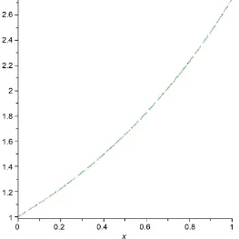
3.2. Model 2: Logistic Differential Equation [15]

( )

(

( )

)

d

1 , 0, 0.

d

u x

u x u x x

(6)

[image:6.595.236.511.72.350.2]

Figure 1. The behavior of the approximate solution and exact solution with m = 5.

We also assume an initial condition

( )

0 0 0.85, 0 0.

u =u = u > (23)

The exact solution to this problem is given by

( ) ( )

0

0 0

.

1 e x

u u x

u −ρ u

=

− +

The procedure of the implementation is given by the following steps: 1) Approximate the function u x

( )

using formula (9)-(14) with m=5

Then the Logistic differential Equation (22) is transformed to the following approximated form

( )

5 5 5

0 0

1 1

0 0 0

1 0.

n n n n n n

n n n

a U∗ x ρ a w x c a w x c

= = =

 

   

− _ + __ −_ + __=

   

∑

(24)

(

m+ =1 6

)

points x_p,p=0,1, 2,3, 4,5 as

( )

5 5 5

0 0

1 1

0 0 0

1 0.

n n p n n p n n p

n n n

a U∗ x ρ a w x c a w x c

= = =

 

   

− _ + __ −_ + __=

   

∑

(25)

For suitable collocation points we use roots of shifted Chebyshev polynomial

( )

6

U∗ x

0 0.96623, 1 0.03377,

x = x =

2 0.38069, 3 0.61930,

x = x =

4 0.16931, 5 0.83060,

(7)

2) Also, by substituting from the initial condition (23) in (18) with u0=0.85

we can obtain

(

k=1

)

an equation which gives the value of the constant

1 0.85

c = .

Equation (25) represents a system of non-linear algebraic equations which contains six equations for the unknowns a n_n, =0,1, 2, 3, 4, 5.

3) Solve the resulting system using the Newton iteration method to obtain the unknowns a n_n, =0,1, 2, 3, 4, 5 as follows

0 1

2 3

6 8

4 5

0.0533, 0.0101, 0.0004, 0.00002,

1.642 10 , 5.398 10 .

a a

a − a −

= =

= − × = ×

(26)

Therefore, from Formula (18) we can obtain the approximate solution in the form

( )

5 ( )0

( )

1 0

n n n

u x a w x c

=

+

∑



( )

2 3 4 5

6 7 8

1 0.5 0.1667 0.0417 0.0083

0.0014 0.0002 0.00004

u x x x x x x

x x x

= + + + + +

+ + +

The numerical results of the proposed problem (22) is given in Figure 2 with

5

m= in he interval [0, 1].

[image:7.595.243.506.425.688.2]

From this Figure 2, since the obtained numerical solutions are in excellent agreement with the exact solution, so, we can conclude that the proposed technique is well for solving such class of ODEs.

(8)

3.3. Model Multi-Order Nonlinear ODEs ([16] [17])

Consider the following initial value problem ([16][17])

( )

3 2 4

2D y x +y x =x (27)

the initial conditions are:

( )

0

( )

0 0,

( )

0 2

y =y′ = y′′ = (28)

1) Approximate the function y x

( )

and its relevant derivatives with k=3

( )

3 ₃ ₃

3 3

0 0

d

d n k k n n n

y x

a p x a w x

x = =

=

∑

 (29)

( )

2 ₃ 2 1 2 0 d

d n n n

y x

a w x c

x =

+

∑



( )

3 ( )1

( )

1 2 0

d

.

d n n n

y x

a w x xc c

x =

+ +

∑



( )

3 ( )

( )

2

0

1 2 3 0 . 2 n n n x

y x a w x c xc c

=

+ + +

∑



where ( )0

( )

( )1

( )

,

n n

w x w x and wn( )2

( )

x are defined as follows

( )

(

)

(

) (

)

0 2 2

0

2 2

1 2

1 2 2 2

n i n

i n i n

i

n i x w x

i n i

− −

=

Γ − +

= −

Γ + Γ − +

∑

( )

(

)

(

) (

)(

)

1

1 2 2

0

2 2

1 2 ,

1 2 2 2 1

n i n

i n i n

i

n i x w x

i n i n i

− + −

=

Γ − +

= −

Γ + Γ − + − +

∑

( )

(

)

(

) (

)(

)

2

2 2 2

0

2 2

1 2 ,

1 2 2 2 1 2

n i n

i n i n

i

n i x w x

i n i n i n i

− + −

=

Γ − +

= −

Γ + Γ − + − + − +

∑

Then the multi-order ODE (27) can be written in the following approximated form

( )

2 2 3 3 0 4

1 2 3

0 0

2

k k n n

n n

x

a p x a w x c xc c x

= =

 

+_ + + + _ =

 

∑

(30)

(

k+1

)

points x_p,p=0,1, 2,3 as

( )

2 2

3 3

0 4

1 2 3

0 0

2

2 p

k k p n n p p p

n n

x

a p x a w x c x c c x

= =

 

+_ + + + _ =

 

∑

(31)

For suitable collocation points we use roots of shifted Chebyshev polynomial

( )

4

p x

2) Also, by substituting from the initial conditions (28) in (29) we can obtain

3

k= of equations which give the values of the constants c c₁, ₂ and c₃.

1 2, 2 0, 3 0.

c = c = c = (32) The Equations (31) and (32) construct system of non-linear algebraic equations which contains seven equations for the unknowns a n_n, =0,1, 2, 3

and c i_i, =1, 2, 3

(9)

Therefore, using the formula (29) we can find the required approximate solution in the following form:

( )

3 ( )

( )

2

0 2

1 2 3 0

. 2

n n n

x

y x a w x c xc c x

=

+ + + =

∑



which is the exact solution of the proposed problem (27).

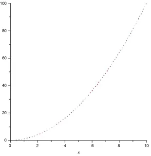
The numerical results of the proposed problem (27) are given in Figure 3 with

5

m= in the interval

[

0,10

]

. From this Figure 3, since the obtained numerical

solutions are in excellent agreement with the exact solution, so, we can conclude that the proposed technique is well for solving such class of ODEs.

4. Conclusion

[image:9.595.219.530.384.706.2]

In this paper, the Chebyshev polynomials of the second kind has been successfully applied to study the model nonlinear ODEs. The results show that Chebyshev polynomials of the second kind is an efficient and easy-to-use technique for finding exact and approximate solutions for nonlinear ordinary differential equations. The obtained approximate solutions using the suggested method is in excellent agreement with the exact solution and show that these approaches can be solved the problem effectively and illustrates the validity and the great potential of the proposed technique.

(10)

Acknowledgements

Thank you for the referees their efforts. The authors would like to thank Prof. Dr. Ahmed Ahmed Hassan, Department of Mathematics, Faculty of Science, Zagazig University, Zagazig, Egypt which provided support.

References

[1] Boyd, J.P. (2001) Chebyshev and Fourier Spectral Methods. 2nd Edition. Courier Corporation, Dover.

[2] Mason, J.C. and Handscomb, D.C. (2003) Chebyshev Polynomials. Chapman and Hall, Boca Raton.

[3] Azizi, H. and Loghmani, G.B. (2013) Numerical Approximation for Space Fraction-al Diffusion Equations via Chebyshev Finite Difference Method. Journal of

Frac-tional Calculus and Applications, 4, 303-311.

http://fcag-egypt.com/Journals/JFCA/Vol4(2)_Papers/14_Vol.%204(2)%20July%20 2013,%20No.%2014,%20pp.%20303-311..pdf

[4] Azizi, H. and Loghmani, G.B. (2014) A Numerical Method for Space Fractional Diffusion Equations Using a Semi-Discrete Scheme and Chebyshev Collocation Method. Journal of Mathematical and Computational Science, 8, 226-235.

[5] Moneim, I.A. and Mosa, G.A. (2006) Modelling the Hepatitis C with Different Types of Virus Genome. Computational and Mathematical Methods in Medicine, 7, 3-13. https://www.hindawi.com/journals/cmmm/2006/318687/abs/

https://doi.org/10.1080/10273660600914121

[6] Meerschaert, M.M. and Tadjeran, C. (2004) Finite Difference Approximations for Fractional Advection-Dispersion Flow Equations. Journal of Computational and

Applied Mathematics, 172, 65-77. https://doi.org/10.1016/j.cam.2004.01.033

[7] Saadatmandi, A. and Dehghan, M.A. (2010) New Operational Matrix for Solving Fractional-Order Differential Equations. Computers & Mathematics with

Applica-tions, 59, 1326-1236. https://doi.org/10.1016/j.camwa.2009.07.006

[8] Sweilam, N.H. and Khader, M.M.A. (2010) Chebyshev Pseudo-Spectral Method for Solving Fractional Order Integro-Differential Equations. The ANZIAM Journal, 51, 464-475.

https://journal.austms.org.au/ojs/index.php/ANZIAMJ/article/downloadSuppFile/... /605

https://doi.org/10.1017/S1446181110000830

[9] Bhrawy, A.H. and Alshomrani, M.A. (2012) SHIFTED LEGENDRE SPECTRAL METhod for Fractional-Order Multi-Point Boundary Value Problems. Advances in

Difference Equations, 2012, 1-19.

https://pdfs.semanticscholar.org/c3bd/71d221c3e19871fa8ec3c79ae17faf06db42.pdf https://doi.org/10.1186/1687-1847-2012-8

[10] Dehghan, M. and Saadatmandi, A. (2008) Chebyshev Finite Difference Method for Fredholm Integro-Differential Equation. International Journal of Computer

Ma-thematics, 85, 123-130. https://doi.org/10.1080/00207160701405436

[11] Elbarbary, E.M.M. (2003) Chebyshev Finite Difference Approximation for the Boundary Value Problems. Applied Mathematics and Computation, 139, 513-523. https://doi.org/10.1016/S0096-3003(02)00214-X

(11)

https://doi.org/10.1016/j.sigpro.2006.02.007

[13] Rawashdeh, E.A. (2006) Numerical Solution of Fractional Integro-Differential Equ-ations by Collocation Method. Applied Mathematics and Computation, 176, 1-6. https://doi.org/10.1016/j.amc.2005.09.059

[14] Sweilam, N.H., Nagy, A.M. and Sayed, A.A. (2015) Second Kind Shifted Chebyshev Polynomials for Solving Space Fractional Order Diffusion Equation. Chaos, Solitons

& Fractals, 73, 141-147. https://doi.org/10.1016/j.chaos.2015.01.010

[15] Khader, M.M., Mahdy, A.M.S. and Shehata, M.M. (2014) An Integral Collocation Approach Based on Legender Polynomials for Solving Riccati, Logistic and Delay Differential Equations. Applied Mathematics, 5, 2360-2369.

https://doi.org/10.4236/am.2014.515228

[16] Abualnaja, K.M. and Khader, M.M. (2016) A Computational Solution of the Mul-ti-Term Nonlinear ODEs with Variable Coefficients Using the Integral-Collocation- Approach Based on Legender Polynomials. Journal of Progressive Research in

Ma-thematics, 9, 1406-1410.

http://scitecresearch.com/journals/index.php/jprm/article/view/857

[17] Sweilam, N.H., Kader, M.M. and ALBar, R.F., (2007) Numerical Studies for Mul-ti-Order Fractional Differential Equation, Physics Letters A, 371, 26-33.

http://www.scirp.org/journal/ajcm

: 10.4236/ajcm.2017.74028

http://creativecommons.org/licenses/by/4.0/

http://fcag-egypt.com/Journals/JFCA/Vol4(2)_Papers/14_Vol.%204(2)%20July%202013,%20No.%2014,%20pp.%20303-311..pdf

13. https://www.hindawi.com/journals/cmmm/2006/318687/abs/

https://doi.org/10.1080/10273660600914121

https://doi.org/10.1016/j.cam.2004.01.033

36. https://doi.org/10.1016/j.camwa.2009.07.006

https://journal.austms.org.au/ojs/index.php/ANZIAMJ/article/downloadSuppFile/.../605

https://doi.org/10.1017/S1446181110000830

https://pdfs.semanticscholar.org/c3bd/71d221c3e19871fa8ec3c79ae17faf06db42.pdf

https://doi.org/10.1186/1687-1847-2012-8

30. https://doi.org/10.1080/00207160701405436

https://doi.org/10.1016/S0096-3003(02)00214-X

https://doi.org/10.1016/j.sigpro.2006.02.007

https://doi.org/10.1016/j.amc.2005.09.059

147. https://doi.org/10.1016/j.chaos.2015.01.010

https://doi.org/10.4236/am.2014.515228

http://scitecresearch.com/journals/index.php/jprm/article/view/857

https://doi.org/10.1016/j.physleta.2007.06.016