Munich Personal RePEc Archive
Standard Risk Aversion and Efficient
Risk Sharing
Suen, Richard M. H.
University of Leicester
6 September 2018
Online at
https://mpra.ub.uni-muenchen.de/88881/
Standard Risk Aversion and E¢cient Risk Sharing
Richard M. H. Suen
This Version: 6th September, 2018.
Abstract
This paper analyzes the risk attitude and investment behavior of a group of heterogeneous
consumers who face an uninsurable background risk. It is shown that standard risk aversion
at the individual level does not imply standard risk aversion at the group level under e¢cient
risk sharing. This points to a potential divergence between individual and collective portfolio
choices in the presence of background risk. We show that if the members’ absolute risk
tolerance is increasing and satis…es a strong form of concavity, then the group has standard
risk aversion.
Keywords: Standard risk aversion; E¢cient risk sharing; Background risk; Portfolio
choice.
JEL classi…cation: D70, D81, G11.
1
Introduction
Both conventional wisdom and empirical evidence suggest that people are more reluctant to
invest in risky assets when they face other sources of uninsurable and undesirable “background”
risk (e.g., labor income risk).1 In a seminal paper, Kimball (1993) shows that an expected-utility
maximizer with decreasing absolute risk aversion (DARA) and decreasing absolute prudence
(DAP) will have this type of response to background risk. The combination of DARA and
DAP is referred to as standard risk aversion. In the present study, we ask whether a group
of diverse individuals, who share risks e¢ciently among themselves and make joint investment
decisions, will respond to background risk in the same way. Speci…cally, we want to identify the
conditions under which the group’s preferences (or aggregate utility function) exhibit standard
risk aversion.
It is known that if all members have DARA preferences, then the aggregate utility function
will have the same property.2 However, this is not true in general for DAP, as we will show below.
In other words, standard risk aversion at the individual level is not enough to ensure standard
risk aversion at the group level under an e¢cient risk-sharing arrangement. One implication is
that a group of standard-risk-averse individuals under such arrangement may choose to increase
their exposure to risky assets in the presence of background risk. A speci…c example is shown
in Section 3. In this paper, we ask the question: under what conditions will collective portfolio
choices under background risk be consistent with individual choices? Our main result shows that
if each individual member’s absolute risk tolerance is increasing and satis…es a strong form of
concavity (which implies DAP) then the aggregate utility function is standard. This result has
two other implications on the group’s preferences. Firstly, since standard risk aversion implies
proper risk aversion and risk vulnerability, our result ensures that the group’s preferences will
have these properties.3 Secondly, DAP implies that the aggregate utility function has a negative
fourth derivative.4 Appset al. (2014) show that this property is not guaranteed in general even
if all the members’ utility function have negative fourth derivative.
1See, for instance, Heaton and Lucas (2000) and Paliaet al. (2014) for empirical evidence. 2See, for instance, Haraet al.(2007, p.656) for a formal statement of this result.
3The notions of “proper risk aversion” and “risk vulnerability” are introduced by Pratt and Zeckhauser (1987)
and Gollier and Pratt (1996), respectively.
4This property is often referred to as “temperance.” See, Kimball (1992) and Eeckhoudt and Schlesinger (2006)
2
The Model
Consider a static model with a group made up of N individuals, N being an integer greater
than one. The group has a sure amount of initial wealth W >0;which can be invested in two
assets: a safe asset with a riskless rate of return r > 0and a risky asset with a random rate of
returnR:e Let and W denote, respectively, the amount of risky and safe investment. The
gross return from this portfolio is given by
(W ) (1 +r) + 1 +Re =!+ x;e
where ! W (1 +r)>0and xe Re r is the excess return from the risky asset. The random
variable ex is drawn from a compact intervalX Raccording to some probability distribution.
Apart from the risky investment, the group also faces an exogenous, uninsurable background
risk yein …nal wealth. The background risk is drawn from a compact interval Y R; it can
take both positive and negative values and is statistically independent of x:e5 The probability
distributions of ex and ey are known to all group members, so there is no disagreement in their
probabilistic beliefs. The sum of investment returns and background risk is used to …nance the
members’ consumption. The group as a whole thus faces the following budget constraint:
N
X
i=1
e
ci !+ xe+y;e (1)
where eci denotes member i’s consumption. Each member’s preferences can be represented by
E[ui(eci)];for i2 f1;2; :::; Ng:The utility function ui :R+ !R is at least …ve times
di¤eren-tiable, strictly increasing, strictly concave and satis…es the Inada condition lim
c!0u
0
i(c) =1: We focus on e¢cient decisions made by the group. Speci…cally, the members of the group
col-lectively decide on a level of risky investment( )and an allocation of consumption(ec1;ec2; :::;ecN)
5One example of such background risk is household earnigs risk. In particular, a positive value of eycan be
so as to maximize a weighted sum of their expected utility, i.e.,
N
X
i=1
iE[ui(eci)];
where i>0is the Pareto weight for member i;subject to (1) andeci 0for alli:This problem
can be divided into two parts: First, conditional on and the realization of (ex;ye); the group
solves a resources allocation problem:
b
u(z) max
fec1;:::;ecNg
N
X
i=1
iui(eci); (2)
subject to
N
X
i=1
e
ci z !+ ex+y;e and eci 0 for all i:
For any z > 0; the constraint set of the above problem is compact. This, together with a
continuous and strictly concave objective function, ensures the existence of a unique solution.
The Inada condition ensures that each optimaleci is strictly positive. By the maximum theorem,
the aggregate utility function bu( ) is continuous and each optimal eci can be determined by a
continuous function i(z);known as the sharing rule. By the implicit function theorem, if each
ui( ) is(m+ 1)times di¤erentiable, then both i( ) andub( ) arem times di¤erentiable. Thus,
under our stated assumptions, both i( ) and ub( ) are at least four times di¤erentiable. In
addition,ub( ) is strictly increasing and strictly concave.
The second part of the group problem is to choose the level of risky investment, i.e.,
maxE[bu(!+ ex+ye)]: (3)
Since the optimal choice of all eci must be strictly positive, the group must choose so that
z ! + xe+ey is strictly positive for all possible realizations of (ex;ye): Depending on the
boundary values of X and Y; this can allow for short-selling of the risky asset (i.e., <0) or
short-selling of the safe asset (i.e., > W). Since the objective function in (3) is continuous
3
Standard Risk Aversion of
u
b
For each member i 2 f1;2; :::; Ng; de…ne Ai(c) u00i (c)=u0i(c) as the measure of absolute
risk aversion and Pi(c) u000i (c)=u00i (c) as the measure of absolute prudence. The reciprocal
of Ai(c); denoted by Ti(c); is the measure of absolute risk tolerance. The …rst derivative of
Ti(c) is referred to as absolute cautiousness [see Wilson (1968)]. Since bu( ) is at least four
times di¤erentiable, we can de…ne the corresponding measures, Ab(z);Tb(z) and Pb(z);for the
aggregate utility function. Wilson (1968) shows that there is a close connection between Ti(c),
b
T(z)and i(z):Speci…cally,
0
i(z) =
Ti[ i(z)]
b
T(z) >0 for all i; and (4)
b
T(z) =
N
X
i=1
Ti[ i(z)]: (5)
Di¤erentiating both sides of (5) with respect toz gives
b
T0(z) =
N
X
i=1
0
i(z)Ti0[ i(z)]: (6)
Since PNi=1 0i(z) = 1;the absolute cautiousness of ub( ) can be viewed as a weighted average of
the individuals’ absolute cautiousness (evaluated under the sharing rule).
We now consider the e¤ect of background risk on the group’s investment decision. Note that
the portfolio choice problem in (3) is no di¤erent from the one faced by asingle decision-maker
(normative representative agent) with utility function bu( ): Thus, according to the variant of
Proposition 6 in Kimball (1993, p.610), any independent background risk ye that raises the
representative agent’s expected marginal utility under the optimal choice ;i.e.,
E ub0(!+ xe+ye) E bu0(!+ ex) ; (7)
will lower the absolute value of if and only if bu( )exhibits standard risk aversion, i.e., when
both Ab( ) andPb( ) are decreasing functions.
From (4) and (5), it is obvious that if Ti( ) is an increasing function (or equivalently,Ai( )
is a decreasing function) for alli;thenAb( )must be decreasing. The relation betweenPi( )and
b
Lemma 1 The representative agent’s absolute prudence is given by
b
P(z)
N
X
i=1
0
i(z)
2
Pi[ i(z)]; (8)
with …rst derivative
b
P0(z) =
N
X
i=1
0
i(z)
3
Pi0[ i(z)] +
2 h
b
T(z)i
2
N
X
i=1
0
i(z)
n
Ti0[ i(z)] Tb0(z)
o2
: (9)
Proof of Lemma 1 Di¤erentiating Ti(c) u0i(c)=u00i (c) with respect to c gives Ti0(c) =
1 +Ti(c)Pi(c)for allc >0:The counterpart forbu( )isTb0(z) = 1 +Tb(z)Pb(z)for allz >0:
Substituting these questions into (6), and using PNi=1 0i(z) = 1 gives
b
T(z)Pb(z) =
N
X
i=1
0
i(z)Ti[ i(z)]Pi[ i(z)]:
Equation (8) follows immediately by rearranging terms and applying (4). Next, di¤erentiating
(8) with respect to z gives
b
P0(z) =
N
X
i=1
0
i(z)
3
Pi0[ i(z)] + 2 N
X
i=1
0
i(z) 00i (z)Pi[ i(z)]:
Di¤erentiating (4) with respect to z gives
00
i (z) =
0
i(z)
b
T(z) n
Ti0[ i(z)] Tb0(z)
o
:
Equation (9) can be obtained by combining the last two equations.
Equation (9) shows that the …rst derivative of Pb( ) can be decomposed into two parts:
The …rst part captures the e¤ects of Pi0( ) on Pb0( ): In particular, this term is negative if
all group members have decreasing absolute prudence. The second term captures the
ef-fects due to the heterogeneity in absolute cautiousness across group members. Since Tb0(z)
is the weighted average of fT0
i [ i(z)]gNi=1 under the set of weights f 0i(z)g N
i=1; the expression
PN
i=1 0i(z)
n
Ti0[ i(z)] Tb0(z)
o2
is the variance of absolute cautiousness among the group
mem-bers, which is always positive. Thus, even if all members have DAP preferences, the
z
0 2 4 6 8 10 12
0.11 0.115 0.12 0.125
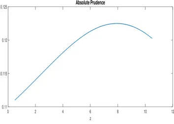
[image:8.595.111.466.89.342.2]Absolute Prudence
Figure 1: An Example of Non-monotonicPb( ):
their risky investment in the presence of background risk. This is demonstrated in the following
example.
Consider two individuals with preferencesu1(c) = 1 1
exp ( c)andu2(c) = c1 1 =(1 );
with >0 and >0: Both individuals exhibit (weakly) decreasing absolute risk aversion and
(weakly) decreasing absolute prudence. When acting alone, the …rst agent’s choice of is
unaf-fected by any background risk that satis…es (7), while the second agent will reduce his/her risky
investment. Suppose now the two form an e¢cient risk-sharing group and suppose 1 = 1:5;
2 = 1:0; = 0:1 and = 0:4: The resulting Pb(z);as depicted in Figure 1, is non-monotonic
and strictly increasing when z is small. Take ! = 4:5 and suppose ex has only two possible
states, -0.2 and 0.24, with equal probability. In the absence of any background risk, the couple’s
optimal choice of risky investment is 1 = 5:093:Suppose now we introduce a background risk
e
y, which can take three possible values: -2.0, 0 and 2.6, with equal probability.6 In the presence
of ye, the couple willincrease their risky investment to 2= 5:105:
The results in our Lemma 1 are closely related to those in Hara et al. (2007, Section
4). Speci…cally, these authors show that e¢cient risk sharing has a tendency to make Tb(z) a
6Condition (7) is satis…ed under thiseyand
1:The detail of this and other parts of the example are shown in
convex function and increase the slope ofTb(z)=z:Thus, even if all group members have concave
absolute risk tolerance or increasing relative risk aversion (which is equivalent to a decreasing
Ti(c)=c), the representative agent may not have these characteristics. The concavity of Tb( ) is
of particular interest here due to the following observation.7
Lemma 2 If Tb( ) is increasing concave, then Pb( ) is decreasing and bu( ) is standard.
Lemma 2 suggests one way to establish the standardness ofbu( ):The remaining question is
under what conditions will Tb( ) be a concave function. Hara et al. (2007) have already shown
that it is not enough to have a concaveTi( )for alli:This prompts us to consider a stronger form
of concavity, which is the notion of “ -concavity” as discussed in Caplin and Nalebu¤ (1991).
For any 2 [ 1;1]; a nonnegative function g( ) is called -concave if the transformed
functioneg(x) [g(x)] = is concave. Since g( )and eg( ) are equivalent when = 1;the usual
notion of concavity corresponds to the case of = 1:8 In general, if g( ) is 1-concave, then
it is also 2-concave for all 2 1: If both g( ) and eg( ) are twice di¤erentiable, then g( ) is
-concave if and only if
g(x)g00(x) (1 ) g0(x) 2; for allx:
The main result of this paper is to show that if each group member’s absolute risk tolerance is
-concave, for some 2;then the representative agent’s absolute risk tolerance is a concave
function. This result holds regardless of whether Ti( ) is monotonic. It follows that if each
Ti( ) is increasing and -concave, for some 2; then Tb( ) is increasing concave and bu( ) is
standard.9
Theorem 3 Suppose for eachi2 f1;2; :::; Ng; Ti( )is -concave, for some 2;thenTb( ) is
a concave function. If, in addition, each Ti( ) is increasing, then ub( ) is standard.
Proof of Theorem 3 As shown in Theorem 4 of Haraet al. (2007), the second derivative of
b
T(z)can be expressed as
b
T00(z) =
N
X
i=1
0
i(z)
2
Ti00[ i(z)] +
1 b
T(z)
N
X
i=1
0
i(z)Ti0[ i(z)]
n
Ti0[ i(z)] Tb0(z)
o
:
7This result has appeared in Gollier (2001b, p.166). Its proof follows immediately by noting thatPb(z)>0;
b
T(z)>0andTb00(z) =Tb0(z)Pb(z) +Tb(z)Pb0(z)for allz >0:
8Quasi-concavity and logconcavity of
Using (4) and (6), we can rewrite this as
b
T00(z) = 1 b
T(z)
N
X
i=1
0
i(z)
n
Ti00[ i(z)]Ti[ i(z)] + Ti0[ i(z)]
2o
h b
T0(z)i2
b
T(z) :
Thus, it su¢ce to show that T00
i (c)Ti(c) + [Ti0(c)]
2
0 for all c 0 and for all i: If Ti( ) is
-concave for some 2;then we haveT00
i (c)Ti(c) (1 ) [Ti0(c)]
2
;which implies
Ti00(c)Ti(c) + Ti0(c)
2
(2 ) Ti0(c) 2 0:
This completes the proof.
In the economics literature, the assumption of -concavity is typically imposed on the density
function of some distributions.10 To the best of our knowledge, this is the …rst study that
applies this type of concavity to characterize risk preferences. Suppose individuals’ absolute risk
tolerance takes a power form as in Gollier (2001a, p.189), i.e.,Ti(c) = ic i;for some constants
i>0and i 0:Then Ti(c)is -concave for some 2 if and only if i 0:5:
1 0For instance, Caplin and Nalebu¤ (1991) impose this assumption on the distribution of voters’ characteristics
References
[1] Apps, P., Andrienko, Y., Rees, R., 2014. Risk and precautionary saving in two-person
households.American Economic Review, 104, 1040-1046.
[2] Caplin, A., Nalebu¤, B., 1991. Aggregation and social choice: a mean voter theorem.
Econometrica, 59, 1-23.
[3] Eeckhoudt, L., Schlesinger, H., 2006. Putting risk in its proper place. American Economic
Review, 96, 280-289.
[4] Ewerhart, C., 2013. Regular type distributions in mechanism design and -concavity.
Eco-nomic Theory, 53, 591-603.
[5] Gollier, C. 2001a. Wealth inequality and asset pricing. Review of Economic Studies, 68,
181-203.
[6] Gollier, C. 2001b. The economics of risk and time. The MIT Press, Cambridge, MA.
[7] Gollier, C., Pratt, J.W., 1996. Risk vulnerability and the tempering e¤ect of background
risk.Econometrica, 64, 1109-1123.
[8] Hara, C., Huang, J., Kuzmics, C., 2007. Representative consumer’s risk aversion and
e¢-cient risk-sharing rules.Journal of Economic Theory, 137, 652-672.
[9] Heaton, J., Lucas, D., 2000. Portfolio choice in the presence of background risk. Economic
Journal, 110, 1-26.
[10] Kimball, M.S., 1992. Precautionary motives for holding assets, in:. Newman, P., Milgate,
M., Falwell, J., (Ed.) The New Palgrave Dictionary of Money and Finance, MacMillan,
London, 158-161.
[11] Kimball, M.S., 1993. Standard risk aversion. Econometrica, 61, 589-611.
[12] Mazzocco, M., 2007. Household intertemporal behaviour: a collective characterization and
a test of commitment. Review of Economic Studies, 74, 857-895.
[13] Ortigueira, S., Siassi, N., 2013. How important is intra-household risk sharing for savings
[14] Palia, D., Qi, Y., Wu, Y., 2014. Heterogeneous background risks and portfolio choice:
evidence from micro-level data.Journal of Money, Credit and Banking, 46, 1687-1720.
[15] Pratt, J.W., Zeckhauser, R.J., 1987. Proper risk aversion. Econometrica, 55, 143-154.