MAINTAINING ATES BALANCE USING CONTINUOUS COMMISSIONING AND MODEL PREDICTIVE CONTROL : Development of a reference model and analysis of method potential based on a case study at the Kropman Utrecht office

MAINTAINING ATES BALANCE USING

CONTINUOUS COMMISSIONING

AND MODEL PREDICTIVE CONTROL

Development of a reference model and analysis of method potential

based on a case study at the Kropman Utrecht office

Master thesis

January 2015

Author:

J.H.K. Hoving

Master Sustainable Energy Technology Eindhoven University (s124057) University of Twente (s0125016)

Department:

Building Services

Unit Building Physics and Services Department of the Built Environment Eindhoven University of Technology (NL)

Graduation committee:

Prof. ir. W. Zeiler Chair of committee Eindhoven University Prof. dr. ir. T.H. van der Meer Program director University of Twente

Ir. J.F.B.C. Haan Company supervisor Kropman Installatietechniek

Dr. R. Li Internal member Eindhoven University

i

A

BSTRACT

A rapidly growing amount of office buildings in the Netherlands is using an Aquifer Thermal Energy Storage (ATES) system. An ATES system uses a well pump to extract cold groundwater for cooling. The returned warm water is injected and stored in a second well. During winter this warm water is used for heating and the returned cold water is injected again in the first well. An optimal functioning ATES system can significantly reduce energy use and CO2 emissions of an office building.

An essential condition for optimal ATES operation is the thermal balance of the system. Office buildings typically store much more heat than cold, causing the entire underground slowly to heat up and causing cooling capacity problems on the long term. This is compensated by using cold outdoor air to store additional cold during the winter, called regeneration. In this research two methods are evaluated to keep the thermal storage in balance. Continuous Commissioning (CC) is used to check if the expected amount of energy is actually stored in the ATES system. Model Predictive Control (MPC) is used to control the amount of regenerated cold to maintain the ATES balance. The key element in both methods is the reference model to calculate the expected stored amount (CC) and use as model for MPC.

A reference model is constructed based on the Kropman Utrecht case study building and contains three main blocks: The ATES, Heating/Ventilation/Air-conditioning (HVAC) and load simulation. For the ATES system a lightweight finite element simulation method is developed, based on an axisymmetric grid. An additional method is developed to reconstruct the injected water temperatures and volumes, because these are not measured in the case study installation. The HVAC and load simulation models are based on logged building management system (BMS) data. The use of BMS data has the large advantage that models are easily configured and can automatically adjust to changes in the building.

The analysis of CC revealed a combination of hardware and software problems. Around 30% of the generated cold is not stored in the ATES system and around 10% of the heat did not need to be stored in the ATES. The use of district heat can be reduced by 60%. Using the current regeneration strategy, the building should generate a significant surplus of cold instead of heat. Using MPC it was possible to keep the ATES in balance over a simulated 20 years period. By using a slight cold surplus as target, the effect of exceptionally warm winters is minimal and extraction temperatures are very constant.

ii

P

REFACE

This thesis is the result of my graduation research for the master Sustainable Energy Technology at the University of Twente. I choose the master SET because I believe the transition from fossil fuels to sustainable energy is one of the largest and most interesting technological challenges the world faces in the coming decades. During the various courses of the master, the sheer size of the sustainable challenge became clear. Sustainable energy is partly about developing and optimizing new technologies, but an even larger challenge is found in integrating all technologies into concepts that provides the same reliability as fossil fuel. A research field that is on the forefront of integrating multiple sustainable technologies into actual systems is building services for the built environment.

Starting this research I had no experience at all in building services. I did a bachelor Applied Physics, so I understood the processes but never saw an actual heat pump or air handling unit. This fresh approach proved to be a bit of a handicap sometimes, but also provided several new insights and proved to be an advantage in ‘out-of-the-box’ thinking. While performing this research one of the main challenges of this field became apparent. Energy is not saved by designing buildings with a reduced energy use, but by making buildings actually save energy. The yearly energy bills represent the buildings energy use and not the framed energy certificate on the wall.

In this research an attempt is done to develop a bridge between the energy bill and the energy certificate. I believe that using methods like continuous commissioning the gap between research, design and reality can be closed and truly sustainable buildings can be constructed. On the other hand I learned to put the challenge for sustainability in perspective. Goals like comfort and reliability are at least equally important and can outweigh the energy efficiency.

Because the University of Twente does not have a building services department, this research is performed under supervision of the Eindhoven University. I would like to thank prof. Wim Zeiler for offering me the opportunity to graduate at this field and supervising the research. I really appreciated the given freedom in performing the research and the provided feedback. The interesting conversations about the construction sector helped me to put the research in perspective.

I also would like to thank my supervisor at Kropman, Jan-Fokko Haan, and all direct colleagues in the O&T team. Every time I had some novice questions you all took the time to give me a crash course on various topics. During the research I was trusted with full access to the BMS and Priva software, the master key of the building and all measurement equipment. This really helped in getting familiar with the building and acquiring the required data. Overall I had a great time at the office in Utrecht.

During the writing of the report I had several interesting meetings at the Eindhoven University. In special I would like to thank Gert Boxem, Rongling Li, Basar Bozkaya and Christian Finck for the discussions and provided help on getting an understandable structure in the thesis.

Finally I would like to thank my parents for supporting me during my time as student. This thesis concludes an exciting and inspiring period at (and around) the University. I’m really grateful for making this possible.

iii

I

NDEX

ABSTRACT ... I

1.

1.1   Background ... 1  

1.2   Problem analysis ... 2  

1.3   Research introduction ... 4  

1.4   Research structure ... 7  

1.5   Case study introduction ... 9  

2.

2.1   Introduction ... 10  

2.2   Aquifer simulation method ... 13  

2.3   Aquifer side data reconstruction method ... 22  

2.4   Implementation of control software method ... 32  

2.5   Discussion ... 37  

3.

3.1   Introduction ... 39  

3.2   Air handling unit simulation method ... 46  

3.3   Local cooling simulation method ... 55  

3.4   Heat pump simulation method ... 59  

3.5   Discussion ... 63  

4.

4.1   Introduction ... 64  

4.2   Load curves reconstruction method ... 64  

4.3   State selection method ... 71  

4.4   Discussion ... 74  

5.

5.1   Continuous commissioning analysis ... 75  

5.2   Model predicitive control analysis ... 80  

5.3   Discussion ... 83  

6.

6.1   Conclusions ... 84  

6.2   Recommendations ... 86  

Page | 1

1. I

NTRODUCTION

1.1 B

The worldwide depletion of fossil fuels, increasing energy prices and climate change have led to sharpened building regulations and the need to design more energy efficient buildings. Buildings constructed during the last decade have high standards of air-tightness and insulation. For all buildings these measures achieve a significant improvement in heating demand and comfort. For office (and comparable) buildings however there is an additional advantage.

Because office buildings typically have a high internal heat load (heat generated by people, lighting and equipment), the required amount of external heat is relatively low compared to residential or utility buildings. As result, the required amount of cooling is significantly higher than the average building. Nowadays modern office buildings have reached the insulation quality at which the amount of cooling required during the summer roughly equals the amount of heating needed during the winter. Hypothetically this means that if all heat could be stored within the building, no external heat source would be needed throughout the year.

The storage of such large amounts of (low quality / temperature) heat within the building would require vast amounts of high heat capacity materials like thick stone walls (as in churches, castles) or phase change materials (PCMs). A more feasible option is to store the energy outside the building. An increasingly popular solution is energy storage in the groundwater below the building. This groundwater is stored in porous sand layers, called aquifers. Therefore, this method is called Aquifer Thermal Energy Storage (ATES). Using this method the seasonal storage effect of an expensive high thermal mass building can be achieved with a cheaper lightweight building construction and an external ATES system.

The principle of an ATES system is based on transferring groundwater between two separated storage wells. During summertime water is extracted from the coldest well and used to cool the building. During cooling, the water temperature increases from approximately 8°C to 16°C. The heated water is injected in the warmer well and stored until winter season. During winter the extraction/injection flow is reversed and the heated water (which still has a temperature of approx. 14 °C) is pumped back to the building. Using a heat pump the heat is extracted and converted to higher temperatures to heat the building. The water is cooled to approx. 6°C and is injected in the cold well. A heat exchanger between the groundwater and the building system water is used to avoid contamination of the water.

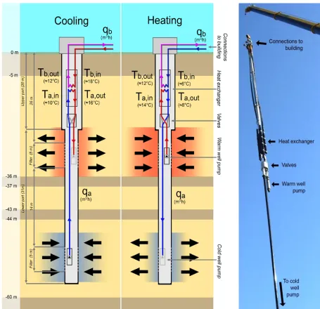
The storage wells can be located horizontally or vertically spaced to each other (Figure 1-1). A horizontally spaced system is called a doublet and has the highest thermal capacity because the total length of the well can be used to inject or extract water. A vertically spaced system is called a mono-well. A mono-well has less capacity, but is significantly cheaper because only one borehole is needed. This research will focus on a mono-well system, as this system is used at the Kropman Utrecht office (the used case study for this research).

Page | 2 For efficient and profitable application of a mono-well ATES system there are a few boundary conditions, which make the Dutch soil structure particularly suitable.

• The groundwater level should be relatively close to the ground level, to avoid expensive

deep drilling. In the Netherlands the groundwater level is usually within 20 meters below the ground level.

• The natural flow in the groundwater should be low to avoid the stored heat/cold flowing away. Due to the flat Dutch landscape, the annual groundwater flow is only a few meters per year.

• To use two vertically spaced wells (a mono-well), there should be an impermeable layer

of clay to avoid a short-cut water flow between the storage wells. A large part of the Dutch soil consists of alternating layers of sand and clay, making it likely that a suitable separation layer can be found.

An optimal performing ATES system can deliver very efficient cooling. The case-study system for example uses a 2 kW well pump that delivers 20 m3/h of cooling water with a ∆T of 8K between extraction and injection. This equals roughly 200 kW of cooling power, a Coefficient of Performance (COP) of 100. For comparison, a regular (compression based) cooling system reaches a COP between 4 and 6 [2]. The energy gains (compared to a conventional system) for heating are not that significant, because the stored low temperature heat is not directly applicable in the building. The heating performance of the ATES system depends mainly on the coupled heat pump, which has a COP of around 4 [2]. However, assuming an average Dutch electricity generation efficiency of 42% [3], this is still a 60% higher efficiency than natural gas boilers and is required to provide the cold water storage supply.

Because of these favorable conditions, the use of ATES systems in the Netherlands has become increasingly popular since the first installations in 1990. In 2013 there were over 2000 installations in use and this number is expected to grow to 10.000 (worst-case) or 20.000 (best-case) in the year 2020 [4].

1.2 P

Although the theoretical performance of ATES systems looks promising, the soil conditions are optimal and the heating and cooling loads of an office building in the Dutch climate are ideal; in reality the performance of the installed systems is not fulfilling expectations. As frequently reported in Dutch newspapers and professional journals [5], [6], [7], the performance of 70% of the ATES systems in the Netherlands is not as successful as designed. Almost 30% of these systems is performing even worse than when conventional heating / cooling methods would be applied [7].

A wide diversity of causes is responsible for these underperforming systems. Based on a selection of case studies [8], [9], [10], articles, experiences of engineers at Kropman and personal experience during the research, an analysis of the main problems is made. These problems can be categorized in four groups (Figure 1-2), depending on the moment in time.

Page | 3

DESIGN CHALLENGES

The design of an ATES coupled Heating, Ventilation and Air Conditioning (HVAC) system is significantly more complex than a conventional system for a number of reasons:

• The extraction temperature of the wells is variable throughout the year

• The typically applied high temperature cooling systems are very sensible to variations in the supply water temperature, because of a small ∆T to the indoor air temperature

• During extraction of warm water simultaneously the cold well must be injected with a

suitable chilled water temperature (and vice versa)

• The ATES-system cannot deliver heating and cooling at the same moment, while

buildings do need simultaneously heating and cooling during spring and autumn. Systems must be designed to optimally buffer and redistribute thermal energy in order to supply a net heating or cooling load to the ATES

• Partial loads (which are already notoriously complex in conventional systems) are even

more complex if also the storage side ∆T must be taken into account

Although engineers are well aware of these complexities, the majority of the systems are designed using a conventional method: Design the installation for full capacity operation during a predefined minimum (for heating) and maximum (for cooling) ambient temperature and assume the system to work between these temperatures (which are by far the most hours per year).

C

The more complex an HVAC system is, the higher the risk of deviations between the original plan and what is actually built. Although a system seems to be quite straightforward on a principle diagram, the actual piping labyrinth of cramped utility rooms can be very confusing. It is not uncommon that systems are not functioning because:

• Advisors, mechanical engineers, software engineers and contractors all use different version of systems drawings.

• Construction mistakes, incorrect connected piping and faulty placed, configured or even

missing sensors and valves.

• Last minute (undocumented) changes in the construction due to problems discovered at

the building site.

Using new techniques like Building Information Modeling (BIM) this should be reduced, but actual construction of the systems shall always be vulnerable to human errors.

O

Because the original performance calculations are made for full capacity operation (for a few hours per year), it is difficult to evaluate how the system is operating during partial load. The dynamic nature of storage based systems causes maintenance difficulties; for example:

• Unlike conventional systems, heating and cooling are always coupled (by both the heat

pump as the storage wells). A problem at the cold-water side of the system can cause heating problems and vice versa.

• A similar difficulty is found in the coupled distribution and storage. A setpoint change of

the distribution (loads) side can significantly influence the stored energy.

• A high number of system states are needed for buffering and redistribution. It can be

difficult to discover which state causes problems under which circumstances.

• Only the problems at the distribution side are noticed directly by a lack of heating or

Page | 4 The fundamental difference between conventional systems and ATES based systems is the ‘charging’ of the storage. This aspect complicates maintenance because of the long-term effects. Imagine for example a technician standing in the utility room of a building during summer season with the assignment to ‘fix the decreased cooling capacity of the ATES’. Obviously this is not possible, because the problems are caused by the lack of stored cold in the winter.

O

The named difficulties in designing, constructing, operating and maintaining an ATES coupled system can be directly connected to problems in optimization of performance. In a system that does not perform as ‘expected’, it won’t be a surprise that optimizations are also not performing as expected. For this reason optimization is often done by trial and error. The system is operated for a few years and after that period the settings are tuned to compensate heat or cold shortage. This requires frequent (and expensive) human intervention in the settings. A few common optimization difficulties are:

• The performance of an ATES system is coupled to the cumulative yearly loads, which

makes it hard to evaluate the optimization results after one rainy summer or a very cold winter. A change in the storage strategy should be evaluated over several seasons to evaluate its results. This makes the trial-and-error method not suitable on short-term.

• If a conventional system has performance problems, a mechanic can solve these

problems within a day of cleaning, repairing, replacing and fine-tuning of the equipment and directly measure the results. Due to the storage aspect, performance optimization can only be measured after several years and the result is highly dependent on climate and building use variations.

In short, it is very complicated (or even impossible) to optimize something when the process that must be optimized is not sufficiently understood and the effects are not directly measurable or predictable.

1.3 R

As can be concluded from the problem analysis, the performance problems of ATES systems are not so much found in the initial hardware design of the ATES and HVAC system (although there is room for improvement). The main problem is found in the understanding, monitoring and prediction of the systems behavior and thermal charging and discharging behavior of the aquifer. To guarantee reliable and robust ATES operation, the storage process must be monitored on short-term events (monitor the past hours/days) and the long-term operation (predict the future months/year). The two analyzed methods to do this are respectively continuous commissioning (short-term) and model predictive control (long-term).

1.3.1 CONTINUOUS COMMISSIONING

Because the long-term performance of the ATES system is the cumulative result of all hour-to-hour events, the key of gaining control over the total stored energy is to monitor each individual event. This can be done by applying a continuous commissioning (CC) system in the building. Continuous commissioning is based on the principle commissioning. This is done when a building is finished and handed over to the owner. All equipment is tested and measured to check if it operates according to the design specifications. CC is an automated real-time version of commissioning to secure that all systems keep operating according to their specifications.

Page | 5 commissioning this can be noticed immediately, while using conventional methods this will be noticed indirectly (and much later) via a cooling capacity shortage, expensive back-up heating energy bills and a thermal ATES imbalance.

It is important to realize continuous commissioning is a concept, not an actual method. Methods for CC are currently under development by several research institutes and for various case-study buildings [11]. However, a uniform method is not yet developed and it still is a kind of ‘umbrella term’ for a large variety of possible implementation methods. One of those methods could be model-based fault detection. As shown in Figure 1-3 this method can compare measured sensor values with a model that simulates ‘correct system behavior’.

Figure 1-3 - The concept of model-based fault detection and its application to a heating coil (from [11])

If a value deviates significantly for a longer time, a warning is generated in the buildings management system (BMS). The main challenge in this method is the development of this ‘correct behavior’ or reference model.

The goal of this research is explicitly not to provide an implementation for the fault detection method. An analysis of the comparison between a reference model and the actual (measured) performance is given. If deviations are caused by actual problems in the system, the fault detection method might be capable of detecting these. The goal of the analysis is to determine if model-based fault detection is a suitable tool to detect ATES-affecting building problems.

1.3.2 MODEL PREDICTIVE CONTROL

Even if (as result of implementing continuous commissioning) the building operates exactly as intended, this does not imply that the ATES will achieve a thermal balance. The stored amounts of energy are influenced by climate variations (i.e. warmer winters) or variations in building use (i.e. internal heat load, building occupancy); these are uncontrollable input variables. For this reason ATES-coupled systems are usually combined with possibilities for regeneration capacity, which supplies additional controllable amounts of energy to the storage to restore balance. The main challenge is to define how much regeneration is required (because of the uncontrollable part) and how to realize it.

Page | 6 umbrella (by using the weather forecast) or the needed force on the brake pedal while driving a car in traffic (by making a prediction of the surrounding cars’ behavior and risks) [13]. Conventional controllers only take the past and current situation in account (find an umbrella when it starts to rain and hit the brake when hitting something).

In Figure 1-4 the basic principle of MPC is shown. An essential component of MPC is the Prediction Horizon. The prediction horizon states within how much time form point ‘k’ the reference trajectory (target state) should be reached. The sample time is the interval between recalculation of the new control inputs.

Figure 1-4 - MPC basic principle [14]

In this research an analysis is made if MPC is capable of maintaining the thermal ATES balance. A reference trajectory is set on the required amount of stored cold during the winter and MPC is used to control the amount of regenerated energy. If the stored amount of cold deviates from the reference trajectory, the control input or regeneration is adapted to reach the reference trajectory within the prediction horizon. A simulated analysis is performed (not an actual implementation) to check if the suggested MPC method is capable of maintaining the thermal balance.

The combination between CC and MPC is essential, because the MPC values are only applicable if the actual system does behave as the reference model suggests. The latter is ensured by implementing model-based CC.

1.3.3 RESEARCH QUESTIONS

Page | 7 This research is based on a case-study building, the Kropman office in Utrecht (NL), of which the ATES system has a structural yearly surplus of stored heat. This results in cooling problems during summer and high-energy use for regeneration. In the original designs a surplus of cold was expected [9], which makes the case-study interesting for both CC as MPC.

The research has two main parts:

1) Model development

How to develop a reference model for the Kropman Utrecht case-study building? Sub questions:

- How to model the ATES system using BMS data? - How to model the HVAC components using BMS data? - How to model the heating and cooling load using BMS data?

2) Model application

Are continuous commissioning and model predictive control suitable tools to maintain the ATES balance of the Kropman building?

Sub questions:

- Which problems could be found by implementing continuous commissioning? - Can model predictive control maintain the ATES balance?

The focus of this research is the development of the reference model, which is the most essential and challenging part.

1.4 R

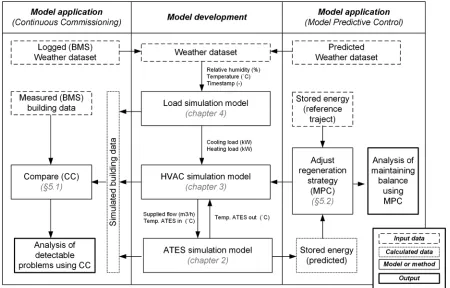
As introduced, this thesis contains two main parts: model development and model application. The main structure is shown in Figure 1-5.

Page | 8

1.4.1 MODEL DEVELOPMENT

To introduce the structure of the developed reference model, only the center column of Figure 1-5 is relevant. The complete reference model is based on three separate models:

1. The load simulation model calculates the heating and cooling loads using the weather data as input.

2. The HVAC simulation model calculates which flows and temperatures are supplied to the ATES as function of the calculated loads and weather conditions.

3. The ATES simulation model calculates the temperature that is supplied back to the building and how the thermal energy is stored in aquifer.

The models are introduced in the reverse order, because this makes it easier to understand how the parts are connected and why certain methods are used.

ATES

In chapter 2 the used ATES model is introduced. A method is presented to simulate the aquifer temperature distribution. Using this method the model can calculate how much energy is stored in the ATES wells and what the expected extraction temperature is. Additional methods are presented to analyze the performance of the well pumps and the heat exchanger. Using a final method that simulates the control software, the entire combination of storage wells, pumps and heat exchanger is simulated. The total model can calculate the outgoing temperature as function of the ingoing temperatures and flows and simultaneously model the effect on the temperature distribution in the storage wells.

HVAC

Chapter 3 introduces the configuration of the buildings HVAC system, how it is operated (the states) and the main components. The system is analyzed from the ATES point of view. All components that do not directly influence the ATES system are left out or simplified using assumptions. The chapter contains three methods to simulate the air-handling unit, the local cooling systems and the heat pump. The focus of these methods is to predict the component behavior mainly based on BMS data, instead of the manufacturers specifications. Using this method, the model can be implemented very easily and eventually monitor or adjust to changing performance over the years.

L

Chapter 4 introduces the developed method to predict how cooling and heating loads are distributed over the buildings HVAC components. Again the modeling methods are based on BMS data to make the model as realistic as possible. It also provides the opportunity to easily readjust the model if parts of the building are not in use. The chapter ends with how the combination of heating curves and load curves influences the selection of system states.

1.4.2 MODEL APPLICATION

Chapter 5 analyses the two applications of the reference model, as showed in the left and right column of Figure 1-5. First continuous commissioning is analyzed by comparing the simulated data with the actual building data. Deviating results are analyzed and the hardware of software related causes are named.

Page | 9

1.5 C

The developed model is based on a case study on the office of Kropman in Utrecht. Kropman is a large HVAC installation company (±800 employees) in the Netherlands with a broad experience on installation, manufacturing, design and ICT solutions. The office in Utrecht houses approx. 150 employees. The building is constructed in 2004 and has a GFA (gross floor area) of roughly 5500 m2_{, which is a typical size of a Dutch office building [15]. The GFA is divided in 3300 m}2 _office space and 2200 m2 _{for storage, restaurant, entree hall and other general spaces. The building} has two wings, both holding 4 floors, which are separated by a large atrium. The atrium is closed in by the wings and two towers containing staircases, elevators, toilets and the majority of the technical installations. The wings contain large open offices with small (meeting) rooms and offices at both ends. Figure 1-6 shows a photo impression of the building.

The building is constructed using the industrial, flexible & demountable (IFD) building method. Buildings constructed with the IFD method are constructed with straightforward industrial methods as a bolted steel frame and prefab concrete floors. The design is based on large open floors without any internal walls. This makes the buildings highly flexible in their use and easy to readjust to future needs.

Figure 1-6 - Impression of the Kropman Utrecht office (offices, restaurant, atrium and outside view)

Page | 10

2. ATES

SYSTEM MODEL

This chapter describes the modeling of the ATES system and includes all components that are inseparably connected to the energy storage process. The chapter starts with an introduction of the system, the problem description and an overview of the used methods. Next the three required methods are introduced to simulate the complete ATES system.

2.1 I

The used mono-well system is the GT-15, which is developed and installed by GeoComfort, a specialized company in ATES systems. The GT-15 is a so-called ‘Turn-key’ ATES system. It is installed as complete integrated solution containing the well, groundwater pumps, heat exchanger, valves, electric hardware and a software system to control the components. First the hardware is introduced followed by the modeling methods of this chapter.

2.1.1 MONO-WELL HARDWARE

The mono-well is constructed using two connected pipes, which form the outer structure of the well. The upper part has a diameter of 0.8 meters and houses the heat exchanger and the valves. The lower part has a diameter of 0.5 meters and houses the two well pumps (schematic overview in Figure 2-1). This pipe contains two filters at the depth of the storage aquifers to prevent sand entering the pumps and water circuit. The entire construction of heat exchanger, valves, pipes and pumps is suspended in the well. Figure 2-2 shows a photo of the actual equipment lifted by a crane during maintenance at the lower well pump (not visible).

The main distinctive feature of a mono-well is the complete system of pumps, valves and heat exchanger operates below natural water level. This way of constructing an ATES system has two advantages. Technically the groundwater is never ‘pumped up’, because the entire process is operated below groundwater level. This simplifies a lot of permit application procedures and also avoids problems with groundwater protection regulations. Secondly, it does have the advantage that the groundwater system is kept under pressure. Because the water pumped from a depth of 50 meters is stored under high pressure, it will release gas when it is depressurized. Below groundwater level the surrounding water pressure prevents this depressurization.

During well drilling the extracted material is analyzed and recorded in the drilling report [16]. The revealed ground structure is shown in Figure 2-1. The yellow layers are sand layers containing the aquifers and the brown layers are the impermeable clay layers that separate the aquifers. The warm and cold storage aquifers are separated by two thin (one meter) clay layers. It could be possible the layers disappear a few meters further away from the well, which causes water flows between the warm and cold well (so-called interference). The drilling report does not provide information about a possible clay layer below the well to seal the lower end of the aquifer. Using a database of ground profiles provided by the Dutch government [17], all surrounding (<1000 meter distance) measurements show a clay layer at 60 meters depth. It is assumed that this layer is also present below the case study well.

Page | 11 counter-flow configuration, which is the most effective way for heat exchange. Table 2-1 introduces the variables of this simulation part. The flow and temperature variables are coded from the heat exchanger point of view; using subscript ‘a’ for aquifer side, ‘b’ for building side, ‘in’ for the incoming stream and ‘out’ for the outgoing stream.

Figure 2-1 – Schematic overview mono-well in heating and cooling mode Figure 2-2 - Picture of ATES installation lifted by a crane

Variable Unit Measured? Description

Ta,in [°C] No Water temperature, aquifer side in (extracted groundwater) Ta,out [°C] No Water temperature, aquifer side out (injected groundwater)

qa [m3/h] No Water flow, aquifer side (controlled by well pump)

Tb,in [°C] Yes Water temperature, building side in (supplied from building system) Tb,out [°C] Yes Water temperature, building side out (returned to building system)

Page | 12

2.1.2 GENERAL SIMULATION METHOD

The main challenge of this simulation part is created by absence of sensors to measure or log data in the groundwater part of the system. The only data known is the percentage of power on which the well pumps are operating (npump), but this value does not provide any direct information without knowing the corresponding flow curve. In essence the goal of this chapter is to model the behavior of the ATES system, without having any measurements of the groundwater system at all.

To create a simulation model of the complete ATES system three methods are developed as shown in Figure 2-3.

Method 1 is the method for the ATES simulation (so only the aquifer storage part) based on data of extracted and injected water data. This data is not available but will be calculated in method 2. This method is explained in section 2.2.

Method 2 is the method to calculate the heat exchanger and well pump characteristics. Using this method the injected and extracted water temperature data for the ATES model (method 1) can be calculated. The method uses all available data logged in the building management system. This method is explained in section 2.3.

Method 3 is the method in which the logged well pump data is replaced by the simulation of the control software. Using this method the return temperature to the building (Tb,out) can be predicted. In the final model the HVAC part (chapter 3) calculates the supplied flow (Qb) and temperature (Tb,in) and this method calculates the return temperature. The method is explained in section 2.4

Page | 13

2.2 A

This section introduces the aquifer simulation method. The goal of this method is to simulate the temperature distribution in the aquifers (and thereby the expected extraction temperatures), as function of the injected water temperatures. This is essential for both the ‘bookkeeping’ of the stored energy as well the behavior of the coupled components. It first explains why a new simulation method is chosen on top of all existing methods, next the calculation method is explained and finally the model is validated.

2.2.1 INTRODUCTION

For the simulation of ATES systems a large variety of methods and software tools is available. To explain why a new method is developed for this research first an analysis of requirements and existing methods is made. The main requirements for the method are:

• A final (long term) goal is to implement the model in the building management software

for the automated monitoring. For this reason specialized commercial (/closed source) simulation software is far from ideal to be used.

• The methods 2 and 3 need the output from the aquifer simulation and vice versa. For this

reason it is highly preferred that both models are simulated in the same simulation software. For the research process preferably MATLAB is used and for future implementation the methods must be translatable to a generic software language.

• Because all logged data points since commissioning (650.000 measurements) should be

included in the simulation to derive the correct aquifer temperature distribution profile, the method must be quite fast.

• For the iterative solving of the problem, the complete 650.000-point dataset must be evaluated numerous times. This requires an even faster simulation tool to create a practical method.

These requirements do narrow the possibilities for an appropriate tool significantly. Roughly, there are three methods to simulate the ATES:

1. Use of open source simulation software with a ‘bridge’ to MATLAB. An example can be the combination of MODFLOW [18] and MFLab [19]

2. Use of a model that is developed natively in MATLAB, like MaxSym [20]

3. Development of a new lightweight simulation model designed specifically for mono-well ATES systems.

Option 1 is not a realistic method, because there should be a continuous data exchange between both programs by exporting and importing data via data files. Even if this only takes a tenth of a second, the processing of the complete dataset will add over a 1000 minutes to the total calculation time. Option 2 is a safe choice, but uses a variety of MATLAB specific functions that would be difficult to transfer to another software language. Based on this analysis, it was worth a try to develop a new method using only the bare essentials needed to simulate the ATES. The next section analyzes which aspects should be simulated for this model.

2.2.2 AQUIFER SIMULATION ASPECTS

Page | 14 simulation, an analysis of the case study mono-well is done, followed by an analysis of the best simulation grid.

S

To make a profound assessment on which simplifications are allowed for the simulation of the aquifer used by the Kropman mono-well, an analysis of the main aspects in groundwater simulation is done.

1) Natural groundwater flow

Natural groundwater flow is caused by a difference in the natural groundwater level, called the hydraulic head. As always in nature, a fluid flows from the highest hydraulic head to the lowest causing natural flow. The differences in hydraulic head can be caused by varying rainwater infiltration or by height differences (mountains). At the Kropman mono-well location the slope in hydraulic head is 13.3 cm/km [26]. Using the hydraulic conductivity of 27 m/day derived in [27], the average natural flow can be calculated at 1.3 meter/year. The storage well area is spread out over an area with a much larger diameter, therefore the effect of groundwater flow is negligible.

2) Hydraulic head variation due to well pumping

When a considerable amount of water is extracted from the aquifer, the hydraulic head will decrease significantly because of a ‘water shortage’ in the pumping zone. For (drinking) water extraction this subsoil water level can drop several meters, making the pump work harder to extract the same amount of water and influencing the flow direction. In the GeoComfort mono-well the flows are relatively small (<20 m3/h) [28] and not continuous. This causes only a drawdown of less than a meter [29] and does not have a significant influence.

3) Flow induced water mixing

During injection and extraction of groundwater, different chemical compositions of groundwater are mixed. For example in mono-well ATES systems, water from a deep aquifer (containing higher amounts of salt) is mixed with water from a less deep aquifer [27]. Although this is an interesting effect, it is highly unlikely to influence the performance of the ATES and thus is not much of interest for this application.

4) Flow induced temperature mixing

When warm water is injected in a colder aquifer, the thermal energy in the water mixes with the existing water and the aquifer sand to reach a new equilibrium temperature. The mixing of different temperature water flows is obviously one of the main processes that determine the temperature profile of the aquifer.

5) Buoyancy effects

Warm water has a lower density than cold water and has the tendency to flow upwards. As investigated in [30] this has a quite significant effect when injecting water of 50 to 90°C. Using water of 30°C the effect is hardly visible. The injected water temperature of the mono-well is around 18°C so the effect is assumed to be negligible.

6) Conduction

Thermal energy storage in an aquifer will require temperature differences between the stored water and the surroundings, which will inevitably lead to conduction losses. Although the temperature differences are relatively small, water and clay are also not very good insulators. This makes conduction also an important factor in ATES simulation.

Overview

Page | 15

S

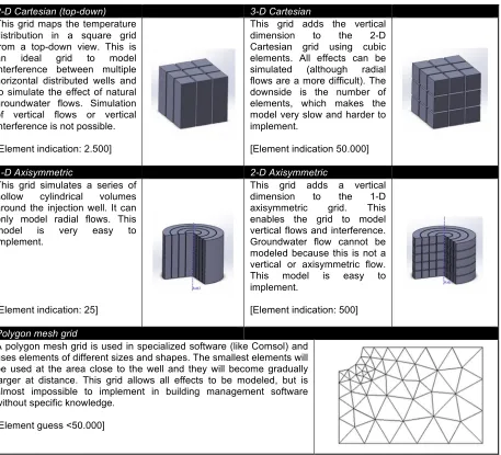
The most common method to simulate the thermal distribution in an aquifer system is to use a finite element simulation. Crucial in the efficiency of design of such a simulation model is the selection of an appropriate grid capable of simulation the essential phenomena. The lowest number of elements will give the fastest model, but can also reduce accuracy. The use of symmetry or reducing dimensions can make the model made faster while sustaining the same accuracy. A selection of commonly used grids is evaluated on their ability to model:

- Radial flows (due to injection or extraction)

- Vertical flows (due to injection in partially penetrated aquifers or buoyancy) - Horizontal flows (natural groundwater flow)

- Interference between axial aligned wells (mono-well configuration) - Difficulty of implementation in building management software

To give an indication of the grid calculation speed, an element number will be given based on a 2 meter grid spacing, 50 meters horizontal range (from well) and 40 meters aquifer thickness. Table 2-2 shows the various possible simulation grids that are commonly used for ATES simulation.

2-D Cartesian (top-down) 3-D Cartesian This grid maps the temperature

distribution in a square grid from a top-down view. This is an ideal grid to model interference between multiple horizontal distributed wells and to simulate the effect of natural groundwater flows. Simulation of vertical flows or vertical interference is not possible.

[Element indication: 2.500]

This grid adds the vertical dimension to the 2-D Cartesian grid using cubic elements. All effects can be simulated (although radial flows are a more difficult). The downside is the number of elements, which makes the model very slow and harder to implement.

[Element indication 50.000]

1-D Axisymmetric 2-D Axisymmetric This grid simulates a series of

hollow cylindrical volumes around the injection well. It can only model radial flows. This model is very easy to implement.

[Element indication: 25]

This grid adds a vertical dimension to the 1-D axisymmetric grid. This enables the grid to model vertical flows and interference. Groundwater flow cannot be modeled because this is not a vertical or axisymmetric flow. This model is easy to implement.

[Element indication: 500]

Polygon mesh grid

A polygon mesh grid is used in specialized software (like Comsol) and uses elements of different sizes and shapes. The smallest elements will be used at the area close to the well and they will become gradually larger at distance. This grid allows all effects to be modeled, but is almost impossible to implement in building management software without specific knowledge.

[Element guess <50.000]

Page | 16

Schematic overview

In Table 2-3 an overview is given of the grids. It is clear that axisymmetric models have the advantage of low element numbers by reducing one dimension using symmetry. The axisymmetric models can simulate radial flow and interference quite simple. The downside is the lacking possibility to simulate the natural flow. The alternatives (the Cartesian grids) perform better at this field, but are performing worse at element numbers (speed). Because natural flow is negligible, the 2-D axisymmetric grid seems to be the best choice.

Cart. (2D) Cart (3D) Axisym. 1D Axisym. 2D Polymesh

Radial flow +/- +/- ++ ++ +

Vertical flow -- ++ -- ++ +

Natural flow ++ ++ -- -- +

Interference -- ++ -- ++ +

Elements 2.500 50.000 25 500 <50.000

Implementation +/- - ++ + --

Table 2-3 - Assessment of simulation grids

2.2.3 AQUIFER SIMULATION METHOD THEORY

There are three sub-methods needed to make this method work. First a method is needed to calculate the flow patterns in a 2D-axisymmetric grid. Next a method is needed to calculate the effect of water mixing with the sand and finally a method to calculate the conduction between the elements. These methods are introduced in this section.

C

A large advantage in the use of an axisymmetric grid (and the neglecting of the horizontal groundwater flow) is found in the fact that the flow pattern can be simplified to a 2D model. A 2- dimensional water flow problem can be solved by calculating the streamlines. Although the water is not flowing freely (in for example a shallow water tank) but through a porous sand structure, the method is still applicable. The sand increases the pressure drop uniformly in all directions, so it does not affect the flow direction.

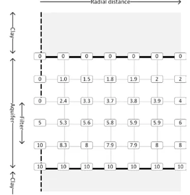
The streamline method is based on the intuitive fact that water will always try to evenly spread out its flow velocity pattern. When this pattern is not averaged out, the velocity differences will create pressure differences. Because water flows always from a higher pressure to a lower pressure, these differences are again directly averaged out. The method is illustrated by Figure 2-4 from (/and further explained in) Fluid Mechanics [31]. In the left figure the boundary values are set. Streamline 0 and 5 follow the impermeable lower and upper boundary, the others are evenly spread between the other grid points on the open left and right end. By iteratively calculating the average of the four neighbors for the other (non boundary) grid points, the streamline distribution can be derived (the right figure).

Page | 17 When the streamline distribution ψ(r,z) is known, the velocity distribution can be calculated using equation 2.1 and 2.2. In the discretized version introduced in Figure 2-4 this can be interpreted as ‘the difference between two points equals the flow between those points’.

𝑈𝑈!= −𝜕𝜕𝜕𝜕_{𝜕𝜕𝜕𝜕      𝑎𝑎𝑎𝑎𝑎𝑎      𝑈𝑈}! =𝜕𝜕𝜕𝜕_{𝜕𝜕𝜕𝜕} (2.1 – 2.2)

To clarify the method for ATES application, an example is given to calculate a 2D axisymmetric flow pattern of a test aquifer. First the boundary values are introduced in Figure 2-5. The streamlines are numbered 0 to 10 (but every range will do) and are linear distributed over the filter length (left side). At the right side a uniform distribution over the whole aquifer thickness is assumed. Streamline ‘0’ follows the upper boundary of the system and streamline ‘10’ the lower. Using the averaging method the values in between are calculated (Figure 2-6).

Figure 2-5 - Streamline method - Boundary values Figure 2-6 - Streamline method - Averaging method

Figure 2-7 shows the calculated streamlines (with .5 interval), only to visualize the stream pattern. By taking the difference between the streamline values on the grid points, the flows are calculated (Figure 2-8). The conservation of water mass within each element is clearly present.

Figure 2-7 - Streamline method – Visualization of

Page | 18

A

When water flows between grid elements, the amount of energy transported depends on the transported amount of water and temperature difference between these elements. For each element the ingoing and outgoing energy is calculated using the flow patterns and the element temperatures calculated in the previous iteration (Figure 2-9).

Figure 2-9 - Energy flow between grid elements

The new temperature can be calculated using an energy balance (equation 2.3). The equation calculates the original energy content of the element, sums the energy content of all ingoing flows, distracts the outgoing flows and calculates the new temperature based on the new element energy content. The energy content of the flow is calculated by multiplying the flow (Qin), temperature (T), timestep (t) and volumetric heat capacity of water (Cwater). The variables used in this equation are shown in table 2.3.

𝑇𝑇!"#=𝑇𝑇!"#∗ 𝑉𝑉 ∗ 𝐶𝐶!"#$+ 𝑄𝑄!",!∗ 𝑡𝑡 ∗ 𝑇𝑇_{𝑉𝑉 ∗ 𝐶𝐶}!∗ 𝐶𝐶!"#$%− 𝑄𝑄!"#,!∗ 𝑡𝑡 ∗ 𝑇𝑇!∗ 𝐶𝐶!"#$%

!"#$ (2.3)

Variable Unit Description

Told/new [°C] The old and new element temperature

V [m3] Element volume

Caqui [MJ/m3K] Specific heat capacity aquifer (sand and water)

Cwater [MJ/m3K] Specific heat capacity water

Qout/in,i [kg/h] Water flow in/out element ‘i’

t [h] Timestep of simulation Ti [°C] Temperature of element ‘i'

Table 2-4 - Variables of equation 2.3

A

For the heat conduction between the elements, a similar method can be applied. The transferred energy depends on the temperature difference, heat conduction and contact area between the elements. The contact area is calculated using equations 2.4 and 2.5 for radial (r) and axial (z) direction.

𝐴𝐴! = 2𝜋𝜋𝑛𝑛!𝑙𝑙!   (2.4)

Page | 19 Using equation 2.6 the thermal resistance between two elements can be calculated. By summing the energy flowing in and out the element, the new temperature can be calculated (equation 2.7). The used variables are introduced in Table 2-1, except the ones that are already used in equation 2.3.

𝑅𝑅! =𝜆𝜆_{𝑙𝑙 ∗ 𝐴𝐴}! ! (2.6)

𝑇𝑇!"#=

𝑇𝑇!"#∗ 𝑉𝑉 ∗ 𝐶𝐶!"#$+ 𝑇𝑇!"#_𝑅𝑅− 𝑇𝑇_! ! 𝑉𝑉 ∗ 𝐶𝐶!"#$

(2.7)

Variable Unit Description

nr [-] Element number in radial direction

λi [W/mK] Thermal conductivity between elements

l [m] Grid size (distance between elements) Ai [m2] Contact area between elements

Ri [W/K] Thermal resistance between elements

Table 2-5 - Variables of equation 2-4 to 2-7

2.2.4 ATES MODEL CONFIGURATION

In section 2.2.3 the general theory is introduced to model an ATES system using the streamline method. This section introduces the configuration to adjust this model to the mono-well system used at Kropman.

First the dimensions of the simulation grid are defined. The soil layers are based on the drilling profile used during construction of the well [16]. The grid is based on a grid size of 2 meters, which is empirically chosen. A smaller grid (1 meter) increases the calculation time with a factor 4 without improving accuracy. A larger grid size (5 meter) smoothens the short-term storage effects (during spring and autumn) too much because of the large volume of the first elements. Table 2-6 shows the used dimensions. The cold aquifer bottom and simulation depth are an estimate based on other (deeper) drillings in the close proximity, because they are not defined in the drilling profile. The simulation length is defined by analyzing at which radial distance there the thermal influence of the ATES is negligible according to the simulation.

Variable Value [m] Grid point

Top warm aquifer 7 4

Top filter warm well 25 13 Bottom filter warm well 31 16 Bottom warm aquifer 35 18 Top cold aquifer 45 23 Top filter cold well 45 23 Bottom filter cold well 51 26 Bottom cold aquifer 57 29 Simulation depth 64 32 Simulation length 60 30

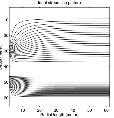
Page | 20 Using the defined grid dimensions, the ideal flow pattern can be calculated (Figure 2-10). The constructed m-file is also capable of simulating interference flows (Figure 2-11). In order to realize this the boundary streamline values (as introduced in 2.2.3) are changed to allow an adjustable fraction of the streamlines going through the clay layer and the remainder via the aquifers. Because the pressure difference between both aquifers decreases with 1/r, the streamlines are distributed with this ratio.

Figure 2-10 - Streamlines of ideal ATES Figure 2-11 - Streamline pattern with interference

The calculation method introduced in section 2.2.3 needs three soil specific properties: the heat capacity of the various layers, the conduction between these layers and the natural temperature distribution. The used heat capacities and conductivities are based on a similar Dutch ATES system used for a research project [32] (Table 2-7).

Description Variable Value Unit Volumetric heat capacity water CH2O 4.2 [MJ/m3K]

Volumetric heat capacity sand Csand 1.5 [MJ/m3K]

Volumetric heat capacity clay Cclay 2.5 [MJ/m3K]

Porosity aquifer n 0.35 [-]

Conductivity aquifer λaqui 2.5 [W/mK]

Conductivity clay λclay 1.7 [W/mK]

Table 2-7 - Heat capacity and conduction values [32]

The volumetric heat capacity of the aquifer layer can be calculated by using the ratio between water and sand (equation 2.8). For the conductivity between a layer of sand and a layer of clay the average conductivity is used.

𝐶𝐶!"#$ = 𝑛𝑛 ∗ 𝐶𝐶!!!+ 1 − 𝑛𝑛 ∗ 𝐶𝐶!"#$ _(2.8)

For the start of the simulation the natural temperature distribution is needed. This is the original distribution of temperatures over the grid elements before the ATES was used. The top layer of soil has on average the same temperature as the average yearly outdoor temperature, which is 10.4 °C [33]. For every 100 meter depth, the soil temperature increases with 2°C [32] as result of heat flowing from the core of the earth. The natural temperature as function of the depth (z) is calculated using equation 2.9.

𝑇𝑇!"# = 𝑇𝑇!"#$+ 0.02𝑧𝑧 (2.9)

Radial length (meter)

Depth (meter)

Ideal streamline pattern

10 20 30 40 50 60

10 20 30 40 50 60

Radial length (meter)

Depth (meter)

Streamline pattern interference

10 20 30 40 50 60

Page | 21 The last step is the definition of the boundary values of the temperature distribution as shown Figure 2-12. The conduction between the upper layer and the outdoor temperature is used to define the temperature of the first elements. For the lower layer a constant temperature based on equation 2.9 is assumed. The last vertical row of elements is defined by only calculating the effects in z-direction and is not influenced by radial (storage) effects. This row simulates the natural surrounding water temperature of the ATES.

2.2.5 METHOD RESULTS

The best way to evaluate and validate the results of this method is to use a dataset of injection and extraction temperatures and compare them to the extraction temperatures predicted by the method. Because there are no aquifer side temperatures and flow data available, this is not possible for the case-study system. A dataset of another building (the ING-House in Amsterdam) is used to check the accuracy of the method. Although this is a doublet system (two separate wells) the calculation method is similar. To avoid confusion by introducing a different ATES configuration the simulation is presented in Appendix A. As shown in Figure 2-13 the results are in general accurate within ± 0.2 °C, except for a few deviations caused by start/stop cycles and low flow. If the ground water is not extracted continuously and at high flow, it exchanges heat to the surrounding soil and causes deviations in the measurements. The average accuracy is sufficient for this research. Simulation of these 5 years of data (300.000 values) takes roughly 30 seconds, which is suitable for the intended purpose.

Figure 2-13 - ATES simulation results ING-House

Fixed temperature Conduction to outdoor

temperature N at ur al tem per at ur e di str ibut ion (onl y ef fec ts i n z -di rec tion )

Page | 22

2.3 A

The developed ATES model is only of use when the injection and extraction temperatures and flows are known. This section introduces the method how this data can be reconstructed. First the available dataset and the interpretation method is introduced. Next the reconstruction method and the corresponding calculation methods are presented. As result the reconstructed characteristics are presented and the accuracy is evaluated.

2.3.1 DATASET HANDLING

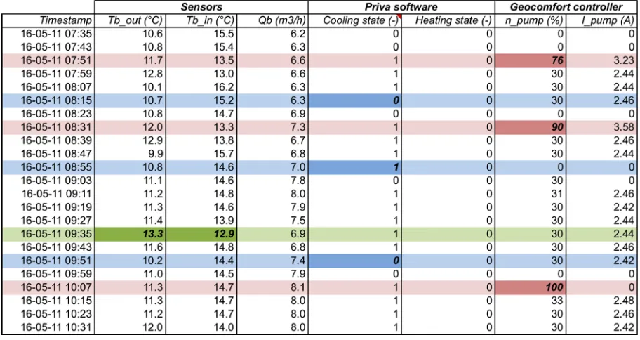
The building management software InsiteView has recorded the sensors monitoring the ATES system every 8 minutes since 2004. A short example of the dataset is shown in Table 2-8. Only the measured value at the sampling moment is stored, so no averaging or filtering is applied. An iteration of storing all values of the BMS takes around 5 minutes, so the values stored for the specific ‘timestamp’ are not recorded at the same moment. The storage order or time offset is not known. There are a few additional remarks on the dataset:

- The values ‘Tb_in’, ‘Tb_out’ and ‘Qb’ are directly logged by InsiteView and should be seen as reference. Although this is the most complete dataset, it has also unexpected values. As marked in green, ‘Tb_out’ is higher than ‘Tb_in’ while the other data suggests the system is continuously in cooling mode.

- The bits ‘Heating’ and ‘Cooling’ are also directly logged, but there is a delay between sending the bit and starting or stopping the well pump (as marked in blue).

- The pump percentage and current are logged by the GeoComfort controller and are extracted by InsiteView. Also those values do not always match each other, have a timestamp mismatch or are missing data due to data extraction errors). It is also unknown which pump (warm/cold well) is active (marked in red).

- The well pumps always start at 100% and slowly lower the flow to the required value. Those startup values are not representative of the effective groundwater flow (marked in

red).

In short, there is data available about the well pumps operation, but this data should be used with great care and must be filtered for steady states based on the temperature and flow data. However, this data sample is an example of start/stop behavior. During continuously cooling (summer) or heating (winter) the data is more consistent.

Page | 23 To find out in which state the mono-well is operating, the building side flow data is filtered using these conditions:

• Cooling state is active if:

o The building-side flow (qb) is > 2 [m3/h]

o The supplied temperature (Tb,in) is > 12 °C

o The temperature difference over the ATES (Tb,in - Tb,out) is at least 1 °C

• Heating state is active if:

o The building-side flow (qb) is > 2 [m3/h]

o The supplied temperature (Tb,in) is < 10 °C

o The temperature difference over the ATES (Tb,out - Tb,in) is at least 1 °C

• Otherwise the system is in rest state and the data is ignored

For every time a heating or cooling state is started (after rest), 0.8 m3 is transferred between the wells to compensate for the full capacity well pump startup flows (as explained in Appendix B).

2.3.2 RECONSTRUCTION METHOD

For the modeling of the integrated mono-well system, three sub-models are needed: 1. A curve to relate the pump flow (qa) to the capacity percentage (npump).

2. A curve to relate the building flow (qb) to the heat transfer function of the heat exchanger 3. The model of method 1 that models extraction temperatures (Ta,in) of the ATES.

These three sub-models all have the problem they can only be calculated (1 & 2) or evaluated (3) when the other two are known. The method used in this part is based on iteratively comparing assumed characteristics with calculated characteristics. When the assumptions for all sub-models correspond with the calculated values (so an iteration of the three steps) without the need to adjust any assumption) the combination is assumed to be correct. There is no hard evidence that these are the actual characteristics, only that the combination of assumptions forms a solution to the problem. Because there are three ‘unknowns’, three calculation steps are needed to evaluate the assumed values. This section introduces the calculation structure. The required background and equations are introduced in the next section (2.3.3).

Step 1. Calculate well pump flow as function of the well pump percentage

The diagram in Figure 2-14 shows the structure of this first step. Using assumptions for the ATES groundwater model, the extracted water temperature (Ta,in) is given. Using assumptions for the heat transfer coefficient and the logged building side water flow data, Ta,out and qa is calculated. By plotting this groundwater flow (qa) as function of the well pump frequency (npump), the flow function is derived. Also Ta,out and qa are used as input for the ATES model, to calculate the new groundwater temperature distribution.

Page | 24

Step 2. Calculate heat transfer coefficient

Figure 2-15 shows the structure used for step 2. Using the previously derived pump flow curve and the pump data (percentages) the heat transfer coefficient curve of the heat exchanger can be calculated. In first sight it may look like this method reconstructs the heat exchanger assumption (circular reasoning), because it uses the same groundwater flows. In reality however the groundwater flows calculated in the first step are very scattered. The well pump linearization produces much more realistic and accurate flow data. The goal of this step is to (iteratively) find the best match between flow characteristics and heat transfer coefficient. Every time the heat transfer coefficient is adjusted, the whole ATES model must also be recalculated because it also influences the injection temperature.

Figure 2-15 - Method to calculate the heat transfer coefficient

Step 3. Evaluate ATES groundwater model input

The third step is to use both the results of step 1 and 2 to reconstruct the extracted water temperature and compare it to the predicted extraction temperatures. Deviation at the start of the heating or cooling season can indicate a wrong calculated injection temperature (defined by the heat exchanger). Deviations at the end of the season (when storage is empty) can indicate the need to adjust the interference.

Figure 2-16 - Method to reconstruct extracted water temperatures

Page | 25

2.3.3 CALCULATION METHODS

The reconstruction method is based on calculations on the heat exchanger. The heat exchanger used in the mono-well is a plate heat exchanger and is used in counter-flow configuration. This section introduces the fundamental physics of a heat exchanger and three calculation models for the steps used in the method.

H

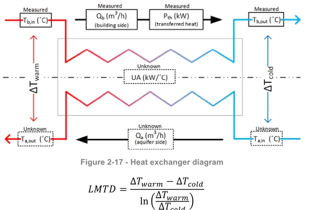
The transferred heat in a heat exchanger can be described by two aspects: the temperature difference between both sides and the thermal conductivity or heat transfer function. The temperature difference is defined using the logarithmic mean temperature difference method (LMTD). The LMTD is calculated using equation 2.10, using the temperature difference at the warm side (∆Tw) and the cold side (∆Tc) (as in Figure 2-17).

Figure 2-17 - Heat exchanger diagram

𝐿𝐿𝐿𝐿𝐿𝐿𝐿𝐿 =Δ𝑇𝑇!"#$− Δ𝑇𝑇!"#$ ln Δ𝑇𝑇!"#$

Δ𝑇𝑇!"#$ (2.10)

Using the LMTD, the transferred heat (kW) is calculated using equation 2.11. The unknown variables in this calculation are the thermal transfer coefficient (U) times the heat exchanger internal conduction area (A). The area (A) is a constant value and the transfer coefficient (U) is defined by equation 2.12 from [34] .

𝑃𝑃!!= 𝐿𝐿𝐿𝐿𝐿𝐿𝐿𝐿 ∗ 𝑈𝑈 ∗ 𝐴𝐴 (2.11)

1 𝑈𝑈 =

1 ℎ!,!"#$%#&'+

1 ℎ!!"+

1

ℎ!,!"#$%&' (2.12)

This equation shows the overall heat transfer coefficient is based on three components:

• ht,building Conductivity between building side water and heat exchanger material

• hhex Conductivity through the heat exchanger material

• ht,aquifer Conductivity between heat exchanger material and aquifer side water

The hhex factor is a constant, depending on the material and thickness of the heat exchanger. The

Page | 26

H

As introduced in section 2.3.2, there are three methods needed to calculate or reconstruct the missing values for the ATES model.

Step 1. Calculation of injection temperature and flow

The first method is the method to calculate the aquifer side flow (Qa) and aquifer injection temperature (Ta,in) as shown in Figure 2-18. All building side values are measured and assumptions are used for the UA value and the extraction temperature.

Figure 2-18 - Heat exchanger calculation - Method 1

Using equation 2.13 the LMTD is calculated and because the Ta,out is the only unknown in equation 2.10, this can be solved by rewriting equation 2.10 to equation 2.14. The resulting aquifer side flow is calculated using ∆Ta and Pth.

𝐿𝐿𝐿𝐿𝐿𝐿𝐿𝐿 =𝑃𝑃_{𝑈𝑈𝑈𝑈}!! (2.13)

𝑇𝑇!,!"# = 𝑇𝑇!,!"+ 𝐿𝐿𝐿𝐿𝐿𝐿𝐿𝐿 ∗ 𝑊𝑊 −𝑒𝑒!!!

!"#$

!"#$ ∗Δ𝑇𝑇!"#$

𝐿𝐿𝐿𝐿𝐿𝐿𝐿𝐿 (2.14)

In equation 2.14 the Lambert W function W(x) is used ( Y = X*exp(X) solves to X = W(Y) ) and is needed to solve the natural logarithm in equation 2.10. The Lambert W function has several branches of solutions, of which -1 and 0 are the primary solutions. As visible in Figure 2-19 the function is only continuous if switched between branches at x = (-1)*exp(-1). For equation 2.14, the following ‘if-statement’ is used:

• If ∆Tcold > LMTD ! Use the 0th branch

• If ∆Tcold = LMTD ! The solution if W(x) = -1

• If ∆Tcold < LMTD ! Use the -1th _branch

Page | 27

Step 2. Calculation of UA factor

The calculation of the UA factor is done using the aquifer flow (Qa) calculated using the well pump percentages (Figure 2-20). Via the energy balance the temperature of the injected water (Ta,out) can be calculated. Because now all temperatures are known, the LMTD can be calculated using equation 2.10 and the UA-value via equation 2.13.

Figure 2-20 - Heat exchanger calculation - Method 2

Step 3. Reconstruction of extracted water temperature

For reconstruction of the temperature of extracted water (Ta,in) the flow is calculated using the well pump percentage (Figure 2-21). Because the flow and transferred heat are known, the temperature difference over the aquifer side (∆Ta) can be calculated.

Figure 2-21 - Heat exchanger calculation - Method 3

Equation 2.15 and 2.16 prove that the difference between the warm/cold side ∆T values equals the aquifer/building side ∆T values. This difference is named ∆Trel, the relative temperature difference, and can be substituted in the LMTD equation (2.17) and solved to equation 2.18. Once ∆Tcold is known, the other temperatures can be solved using energy balances.

Δ𝑇𝑇!+  Δ𝑇𝑇!"#$ = Δ𝑇𝑇!+  Δ𝑇𝑇!"#$ (2.15)

Δ𝑇𝑇!− Δ𝑇𝑇! =  Δ𝑇𝑇!"#$−  Δ𝑇𝑇!"#$= Δ𝑇𝑇!"# (2.16)

𝐿𝐿𝐿𝐿𝐿𝐿𝐿𝐿 =Δ𝑇𝑇!"#$− Δ𝑇𝑇!"#$ ln Δ𝑇𝑇!"#$

Δ𝑇𝑇!"#$

=   Δ𝑇𝑇!"# ln Δ𝑇𝑇!"#$+ Δ𝑇𝑇!"#

Δ𝑇𝑇!"#$

(2.17)

Δ𝑇𝑇!"#$ = Δ𝑇𝑇!"#