http://wrap.warwick.ac.uk/
Original citation:
Masood, K., Rajpoot, Nasir M. (Nasir Mahmood), Qureshi, H. and Rajpoot, K. (2006)
Co-occurrence and morphological analysis for colon tissue biopsy classification. In: 4th
International Workshop on Frontiers of Information Technology (FIT 2006), Islamabad,
Pakistan, 20-21 Dec 2006
Permanent WRAP url:
http://wrap.warwick.ac.uk/61551
Copyright and reuse:
The Warwick Research Archive Portal (WRAP) makes this work by researchers of the
University of Warwick available open access under the following conditions. Copyright ©
and all moral rights to the version of the paper presented here belong to the individual
author(s) and/or other copyright owners. To the extent reasonable and practicable the
material made available in WRAP has been checked for eligibility before being made
available.
Copies of full items can be used for personal research or study, educational, or
not-for-profit purposes without prior permission or charge. Provided that the authors, title and
full bibliographic details are credited, a hyperlink and/or URL is given for the original
metadata page and the content is not changed in any way.
A note on versions:
The version presented in WRAP is the published version or, version of record, and may
be cited as it appears here.For more information, please contact the WRAP Team at:
CO-OCCURRENCE AND MORPHOLOGICAL ANALYSIS FOR COLON TISSUE BIOPSY
CLASSIFICATION
Khalid Masood, Nasir Rajpoot, Hammad Qureshi
Department of Computer Science
University of Warwick
Coventry, CV4 7AL, UK
Kashif Rajpoot
Wolfson Medical Vision Lab
University of Oxford
UK
ABSTRACT
Diagnosis and cure of colon cancer can be improved by effi-ciently classifying the colon tissue cells from biopsy slides into normal and malignant classes. This paper presents the classification of hyperspectral colon tissue cells using mor-phology of gland nuclei of cells. The application of hyper-spectral imaging techniques in medical image analysis is a new domain for researchers. The main advantage of using hyperspectral imaging is the increased spectral resolution and detailed subpixel information. The proposed classifi-cation algorithm is based on the subspace projection tech-niques. Support vector machine, with 3rd degree polyno-mial kernel, is employed in final set of experiments. Dimen-sionality reduction and tissue segmentation is achieved by Independent Component Analysis (ICA) andk-means clus-tering. Morphological features, which describe the shape, orientation and other geometrical attributes, are extracted in one set of experiments. Grey level co-occurrence ma-trices are also computed for the second set of experiments. For classification, kernel discriminant analysis (LDA) with co-occurrence features gives comparable classification ac-curacy to SVM using a gaussian kernel. The algorithm is tested on a limited set of samples containing ten biopsy slides and its applicability is demonstrated with the help of measures such as classification accuracy rate and the area under the convex hull of ROC curves.
1. INTRODUCTION
Colon cancer is a malignant disease of the large bowel. Af-ter lung and breast cancer, colorectal cancer (a combined term for colon and rectal cancer) is the most common cause of death for cancers in the Western world. The incidence of disease in England and Wales is about 30,000 cases/year, resulting in approximately 17,000 death/annum [11], and it has been estimated that at least half a million cases of col-orectal cancer occur each year worldwide. It is caused by colonic polyps, an abnormal growth of tissue that projects in due course from the lining of the intestine or rectum, into
colorectal cancer. These polyps are often benign and usually produce no symptoms. They may, however, cause painless rectal bleeding usually not apparent to the naked eye. The normal time for a polyp to reach 1 cm in diameter is five years or a little more. This 1 cm polyp will take around 5-10 years for the cancer to cause symptoms by which time it is frequently too late [10].
Diets low in fruits, less protein from vegetable sources, high age and family history are associated with increased risk of polyps. Persons smoking more than 20 cigarettes a day are 250 percent more likely to have polyps as opposed to nonsmokers who otherwise have the same risks. There is an association of cancer risk with meat, fat or protein con-sumption which appear to break down in the gut into cancer causing compounds called carcinogens [8]. Smoking ces-sation is important to decrease the likelihood of developing colon cancer. Dietary supplementation with 1500 mg of cal-cium or more a day is associated with a lower incidence of colon cancer. Weight reduction may be helpful in reducing the risk for colorectal cancer. Daily exercise reduces the likelihood of developing colon cancer. Turmeric, the spice which gives curry its distinctive yellow color, may also pre-vent colon cancer [5].
1.1. Hyperspectral Imaging
Hyperspectral imaging in laboratory experiments, is a non-contact sensing technique for obtaining both spectral and spatial information about a tissue sample. Hyperspectral imaging measures a spectrum for each pixel in an image. There are many types of spectroscopy which are being used to study the spectral signatures of individual cells and un-derlying tissue sections. In optical spectroscopy, which mea-sures transmission through, or reflectance from, a sample by visible or near-infrared radiation at the same wavelength as the source, classification is done mostly by statistical mea-sures [1].
materials and its variation in energy with wavelength [9]. Spectrometers are used to make measurements of the light reflected from a test specimen. A prism in the centre of spectrometer splits this light into many different wavelength bands and the energy in each band is measured by detectors which are different for each band. By using large number of detectors (even a few thousand), spectrometers can make spectral measurements of bands as narrow as 0.01 microm-eters over a wide wavelength range, typically at least 0.4 to 2.4 micrometers (visible through middle infrared wave-length ranges). Most approaches to analyse hyperspectral images concentrate on the spectral information in ual image cells, rather than spatial variations within individ-ual bands or groups of bands. The statistical classification (clustering) methods often used with multispectral images can also be applied to hyperspectral images but may need to be adapted to handle high dimensionality.
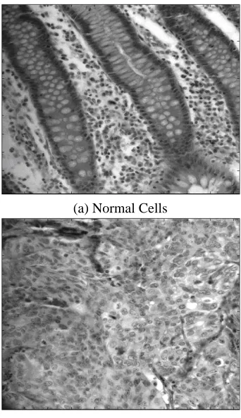
Recent developments in hyperspectral imaging have en-hanced the usefulness of the light microscope [3]. A stan-dard epifluorescence microscope can be optically coupled to an imaging spectrograph, with output recorded by a CCD camera. Individual images are captured representing Y-wave-length planes, with the stage successively moved in the X di-rection, allowing an image cube to be constructed from the compilation of generated scan files. Hyperspectral imaging microscopy permits the capture and identification of differ-ent spectral signatures presdiffer-ent in an optical field during a single-pass evaluation, including molecules with overlap-ping but distinct emission spectra. High resolution charac-teristics of hyperspectal imaging is reflected in two sample images in Figure 1 of colon tissue cells.
2. DIMENSIONALITY REDUCTION AND SUBSPACE PROJECTION
There is a large redundant information in the subbands of hyperspectral imagery. Independent component analysis (ICA) is used to discard the redundancy and extract the variance among different wavelengths of spectra. K-means cluster-ing is used to help the dimensionality reduction procedure and to segregate the biopsy slide into its cellular compo-nents. Subspace projection is achieved with principal com-ponent analysis (PCA) and linear discriminant analysis (LDA). A brief introduction to the mathematical derivation of these methods is presented in the following subsections.
2.1. Independent Component Analysis (ICA)
The objective of Independent Component Analysis (ICA) is to perform a dimension reduction approach to achieve decorrelation between independent components [14]. Let us denote byX = (x1, x2, . . . , xm)
T
a zero-mean m-dimensional variable, andS = (s1, s2, . . . , sn)
T
,n < m, is its linear
(a) Normal Cells
[image:3.612.342.513.70.367.2](b) Malignant Cells
Fig. 1. Colon Tissue Imagery
transform with a constant matrixW [17]:
S=W X
Given X as observations, ICA aims to estimating W and S. The goal of ICA is to find a new variable S such that trans-formed componentssiare not only uncorrelated with each
other, but also statistically as independent of each other as possible. An ICA algorithm consists of two parts, an ob-jective function which measures the independence between components, entropy of each independent source or their higher order cumulants, and the second part is the optimisa-tion method used to optimise the objective funcoptimisa-tion. Higher order cumulants like kurtosis, and approximations of ne-gentropy provide one-unit objective function. A decorrela-tion method is needed to prevent the objective funcdecorrela-tion from converging to the same optimum for different independent components. Whitening or data sphering project the data onto its subspace as well as normalizing its v ariance.
2.2. K-Means Clustering
patterns in the same cluster are alike and patterns belonging to two different clusters are different. Thek-means method has been shown to be effective in producing good clustering results for many practical applications [2]. The aim of thek -means algorithm is to dividempoints inndimensions into
kclusters so that the within-cluster sum of squared distance from the cluster centroids is minimised. The algorithm re-quires as input a matrix ofmpoints in ndimensions and a matrix ofk initial cluster centres inndimensions. The number of clusterskis assumed to be fixed ink-means clus-tering. Let thekprototypes(w1, . . . , wk)be initialised to
one of theminput patterns(i1, . . . , im). Therefore;
wj =il, j∈ {1, . . . , k}, l∈ {1, . . . , m}
The appropriate choice ofkis problem and domain depen-dent and generally a user must try several values ofk. The quality of the clustering is determined by the following error function: E = k X j=1 X
il∈Cj
|il−wj|2
The direct implementation ofk-means method is computa-tionally very intensive.
2.3. Kernel Principal Component Analysis
PCA is a kind of linear transform, while Kernel PCA is a nonliner transform. The basic idea of KPCA [13] is based on the theory that by doing nonlinear mapping of the data points to a higher dimensional space, better features are ob-tained which is more natural and compact representation of the data. The computational complexity arising from the high dimensionality mapping is mitigated by using the ker-nel trick. Consider a nonlinear mappingΦ(.) : Rn →
Rf, f > nthe space of n dimensional data points to some higher dimensional spaceRf. So every pointxnis mapped
to some point φ(xf)in a higher dimensional space.
Af-ter mapping, KPCA is nothing but linear PCA done on the points in the higher dimensional space. Denoting am×
m matrix K by
Kij =k(xi, xj) = Φ(xi).Φ(xj)
the kernel PCA problem becomes
mλkα=k2α≡mλα=kα
whereαdenotes a column vector with entriesα1,· · ·, αm.
The projection vectors inRf to a lower dimensional space
spanned by the eigenvectorswΦ is the nonlinear principal components corresponding toΦ:
wΦ.Φ(x) =
m
X
i=1
αi(Φ(xi)).Φ(x) = m
X
i=1
αik(xi, x)
hence the first m nonlinear principal components are ex-tracted without the expensive operation of high dimensional projection of the data.
2.4. Kernel Linear Discriminant Analysis
Similar to KPCA, mapping is performed on the input space to the high dimensional feature space with linear properties [13]. In the new space, the problem is solved in a clas-sical way in the transformed space using the kernel oper-ators.Denoting the wihin-class and between-class matrices bySw andSb and applying FDA in kernel space, the
so-lution of the equation below will give the eigenvalues and eigenvectors w ;
λSwΦwΦ=SΦBwΦ
which can be obtained by
WOP TΦ =argmaxwΦ
|(WΦ)TSBΦWΦ| |(WΦ)TSΦ
WWΦ|
= [wΦ1,· · ·, wΦm]
. Consider a c-classs problem and let therthsample of class
t andsthsample of class u bextrandxusrespectively. The
kernel function is defined as
(krs)tu=k(xtr, xus) = Φ(xtr).Φ(xus)
. Let K be am×mmatrix defined by the elements(Ktu) t=1,···,c u=1,···,c
where Ktu is a matrix composed of dot products in the
feature space Rf,i.e., K = (K tu)
t=1,···,c
u=1,···,c whereKtu =
(krs) r=1,···,lt
s=1,···,lu. Note Ktu is a lt×lu matrix, and K is a m×msymmetric matrix. We can also define a matrix Z :
Z = (Zt)t=1,···,c
whereZtis am×mblock diagonal matrix. The
between-class and within-between-class scatter matrices in a high dimensional feature spaceRf are defined as;
SBΦ=
C
X
c=1
liµΦi (µ
Φ
i) T
SwΦ=
C X i=1 li X j=1
Φ(xij)(Φ(xij)T
whereµΦi is the mean of class i inRf,li is the number of
samples belonging to class i. From the theory of reproduc-ing kernels, any solutionwΦ ∈ Rf must lie in the span of all training samples inRf,i.e.
wΦ=
C X p=1 lp X q=1
3. METHODOLOGY
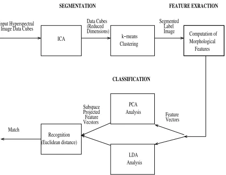
The proposed classification algorithm consists of three mod-ules as shown in Figure 2. Brief description of dimensional-ity reduction and feature extraction modules is given in the following sub-sections. Detailed description of the segmen-tation can be found in [12].
Clustering
LDA Analysis Analysis PCA
Recognition
ICA k−means Computation ofMorphological Features
Feature
SEGMENTATION FEATURE EXRACTION
CLASSIFICATION
(Reduced Dimensions) Data Cubes
Match
(Euclidean distance) VecstorsFeature Projected Subspace
Vectors Segmented Label Image Input Hyperspectral
[image:5.612.51.278.163.339.2]Image Data Cubes
Fig. 2. Classification Algorithm Block Diagram
3.1. Segmentation
High dimensional data in the form of 3-D cubes is obtained using hyperspectral imaging. For efficient processing this data has to be dimensionally reduced. Dimensionality re-duction involves two steps, extraction of statistically inde-pendent components using Indeinde-pendent Component Anal-ysis (ICA) and colour segmentation usingk-means cluster-ing. Flexible ICA (FlexICA) [6], a fixed point algorithm for ICA, adopting a generalised Gaussian density, is used for data sphering (whitening) and achieves considerable di-mensionality reduction. Data is distributed towards heavy-tailedness by the high-emphasis filters. The data with re-duced dimensionality is then fed tok-means clustering al-gorithm for segmentation.
The hyperspectal data cube containing 28 subbands is segmented into four labeled parts. Each slide of the tissue cells is divided into four regions represented by four colours as shown in Figure 3. The four labeled parts are denoted by colours as dark blue for nuclei, light blue for cytoplasm, yellow for gland secretions and red for lamina propria.
3.2. Feature Extraction
3.2.1. Morphological Features
In order for the pattern recognition process to be tractable it is necessary to represent patterns into some
mathemati-(a) Benign Cells
(b) Malignant Cells
Fig. 3. Segmentation Results
cal or analytical model. The model should convert patterns into features or measurable values, which are condensed representations of the patterns, containing only salient in-formation [7]. Features contain the characteristics of a pat-tern to make them comparable to standard templates making the pattern classification possible. The extraction of good features from these pattern models and the selection from them of the ones with the most discriminatory power are the basis for the success of the classification process. In this work morphological texture features, extracted from the segmented images of a hyperspectral data cube for a biopsy slide of colon tissue cells, are used for the classification of the tissue cells.
3.2.2. Co-occurnence Features
The co-coourrence approach is based on the grey level spa-tial dependence. Co-occurrence matrix is computed by second-order joint conditional probability density functionf(i, j|d, θ). Eachf(i, j|d, θ)is computed by counting all pairs of pixels separated by distancedhaving grey levelsiandj, in the given directionθ. The angular displacementθusually takes on the range of values from θ = 0,45,90,135 degrees. The co-occurrence matrix captures a significant amount of textural information. The diagonal values for a coarse tex-ture are high while for a fine textex-ture these diagonal values are scattered. To obtain rotataion invariant features the co-occurrence matrices obtained from the different directions are accumulated. The three set of attributes used in our ex-periments are Energy, Inertia and Local Homogeneity.
E=X
i
X
j
[f(i, j|d, θ)]2
I=X
i
X
j
[(i−j)2f(i, j|d, θ)]
LH=X
i
X
j
f(i, j|d, θ) 1 + (i+j)2
4. EXPERIMENTS
4.1. Experimental Setup
The experimental setup consists of a CRI Nuance micro-scope and a CCD camera. Two different biopsy slides con-taining several microdots, where each microdot is from a distinct patient, is prepared. Then each slide is illuminated with a tuned light source (capable of emitting any combina-tion of light frequencies in the range of 450-850 nm), fol-lowed by magnification to 400 X. Thus several images, each image using a different combination of light frequencies, are produced [4].
The first set of experiments is carried out with mixed training/test data. Each image is divided into 4096 patches of 16×16 dimensions per patch. Morphological opera-tion is performed on the patches for extracopera-tion of feature vectors using different combinations of ten scalar morpho-logical properties. The data (patches of all slides randomly mixed) is divided into training set (about one quarter of the patches) and test set (remaining three quarters of patches). In the other experiment, multiscale feature extraction is per-formed. Feature values are initially calculated for base patch size16×16, patch size is then doubled and feature values are re-calculated. This process continues for at least upto five scales. Fusion of the features, for different scales, is done by simple concatenation. Thus largest feature vector for five scales and using ten morphological parameters has dimensions of 200 fetures values.
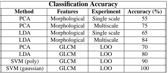
Classification Accuracy
Method Features Experiment Accuracy (%) PCA Morphological Single scale 55 PCA Morphological Multiscale 75 LDA Morphological Single scale 65 LDA Morphological Multiscale 84
PCA GLCM LOO 70
LDA GLCM LOO 80
SVM (poly) GLCM LOO 90
[image:6.612.309.600.71.198.2]SVM (gaussian) GLCM LOO 100
Table 1. Classification Results
4.2. Experiments with Leave one out data
The second set of experiments are used with LOO (leave one out) settings and employing two different subsets. In the second setting, co-occurrence matrix is computed from the block size of 64x64 for each slide. Three co-occurrence features i.e. Angular second moment (Energy), variance and homogenity are calculated while pixel distance is varied from one pixel to two pixel values. Four directional features in the direction of 0, 45, 90 and 135 are concanated together so that feature vector with 24 dimensions is used in the classifiers. The last experiment is carried out with SVMs. Polynomial kernel of 3rd degree with parameters C=1 (cost of constrain violation), epsilon=0.001 (tolerance of termi-nation criterion), and coefficient=0 is used in this exercise. Experiments with SVM using Gaussian kernel have the best classification accuracy of 100 percent for a threshold of 60 percent coorect patches.
4.3. Results
The classification accuracy in GLCM-LOO is about 90 per-cent and 9 slides on the whole are classified correctly with a threshold of 55 percent on the patches. Directly fed patches have a little less performance as compared to the co-occurrence features from the patches. As we have only limited number of input slides, so comparison is difficult on these set of ex-periments. Using new data with these setting will give better comparison for the classification accuracy.
5. CONCLUSIONS
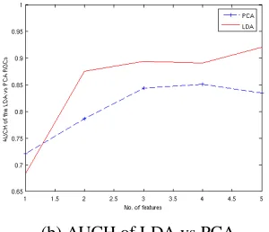
(b) AUCH of LDA vs PCA
Fig. 4. AUCH Performance Curves
malignant tissue. In morphological analysis, five features’ subset is used to achieve 80 percent accuracy. In the second set of experiments with gray level co-occurrence matrix and using a feature vector of 24 dimensions, reasonable classi-fication is performed even with simple classifiers like LDA. However, employing properly tuned Gaussian kernel with grid search method, accuracy level as good as 100 percent can be achieved.
Acknowledgments
The authors are greatly indebted to Gustave Davis, Mauro Maggioni and Ronald Coifman of the School of Medicine and the Applied Mathematics Department of Yale Univer-sity for providing the data and for many fruitful discussions.
6. REFERENCES
[1] John Adams, M. Smith, and A. Gillespie. Imaging spectroscopy: Interpretation based on specral mixture analysis. Remote Geochemical Analysis, 1993.
[2] K. Alsabti, S. Ranka, and V. Singh. An efficient k-means clustering algorithm. www.cise.ufl.edu., 1997.
[3] E. A. Cloutis. Hyperspectral geological remote sensing. Evaluation of Analytical Techniques-International Journal of Remote Sensing, 17:2215–
2242, 1996.
[4] G. Davis, M. Maggioni, and R. Coifman et al. Spec-tral/spatial analysis of colon carcinoma. Journal of
Modern Pathology, 2003.
[5] R. S. Houlston. Molecular pathology of of colorectal cancer. Clinical Pathology, 2001.
[6] A. Hyvarinen. Survey on independent component analysis. Neural Computing Surveys, 2:94–128, 1999.
[7] Anil Jain, Robert Duin, and Jianchang Mao. Statistical pattern recognition: A review. IEEE Trans. on Pattern
Analysis and Machine Intelligence, 22, 2000.
[8] S. Kaster, S. Buckley, and T. Haseman. Colonoscopy and barium enema in the detection of colorectal can-cer. Gastrointestinal Endoscopy, 1995.
[9] David Landgrebe. Hyperspectral image data analy-sis as a high dimensional signal processing problem.
IEEE Signal Processing magazine, 2002.
[10] D. E. Mansell. Colon polyps & colon cancer.
Amer-ican Cancer Society Textbook of Clinical Oncology,
1991.
[11] Office of National Statistics. Cancer statistics: Regis-trations, england and wales. london. HMSO, 1999.
[12] K. M. Rajpoot and Nasir M Rajpoot. Hyperspectral colon tissue cell classification. SPIE Medical Imaging
(MI), 2004.
[13] N. Rajpoot and K. Masood. Human gait recognition with 3-d wavelets & kernel based subspace projec-tions. International Workshop on HAREM, 2005.
[14] Kun Zhang and Lai-Wan Chan. Dimension reduction based on orthogonality-a decorrelation method in ica.