Passive maintenance of high angle of attack and its lift generation during flapping translation in crane fly wing

INTRODUCTION

The unsteady aerodynamic effects that generate lift forces in insect flapping flight depend on the kinematic pattern of the wing pitching motion (Dickinson and Gotz, 1993; Ellington et al., 1996; Dickinson et al., 1999; Birch and Dickinson, 2003). The fundamental features of the kinematic patterns are the maintenance of a high angle of attack of the wing during the flapping translation and the wing rotation during the stroke reversal (see Fig.1). The high angle of attack generates a vortex on the leading edge of the wing (leading edge vortex), which generates a large and instantaneous lift force on the wing. Since the leading edge vortex is reproduced during the next half stroke before the previous vortex separates from the wing, sufficient lift is provided continuously in insect flight. The lift during the stroke reversal is enhanced by circulation effects resulting from the wing rotation. It is therefore important to understand how these fundamental features of the pitching motion are produced.

Although insects regulate the timing of the wing rotation (Dickinson et al., 1993), it seems that the inertial force can cause wing rotation. Ennos (Ennos, 1988b) has suggested using the rigid pendulum model for a dipteran wing that the inertial force of the wing mass is sufficient to account for much of the rotation. Bergou et al. (Bergou et al., 2007) also studied the inertial cause of the wing rotation in some different insects (dragonflies, fruit fly and hawkmoth) using the flapping wing section model and computational fluid dynamics and found that the inertial force of the wing mass and the added mass from air is sufficient to cause the wing rotation in all tested insects.

Morphological studies on the dipteran wings have shown that there exists high torsional flexibility concentrated on the wing basal region (Ennos, 1987; Ennos, 1988a). This flexibility might prevent

insects from transmitting the active torsional force applied by their own muscle to the outer wing. It has been suggested that the aerodynamic pressure is sufficient to produce the observed torsion using the static linear relation between the assumed aerodynamic pressure and the torsional stiffness of the wing (Ennos, 1988a). In our previous study (Ishihara et al., 2009), we used the flapping wing section model with a spring to model the wing torsional flexibility, and the finite element method to analyze the motion of the model wing interacting with the surrounding fluid. Under the dynamic similarity between the crane fly flight and our model flight, our model wing passively maintained a high angle of attack during the flapping translation and rotated quickly upon the stroke reversal without any prescribed pitching motion. The lift force generated by such passive pitching was comparable with but smaller than the weight of the crane fly. This could be attributed to the loosely attached leading edge vortex on the wing that resulted from the long wing chord travel of the crane fly for the two-dimensional simulation. In addition, it was not clear what forces are important for the production of the features of pitching motion. Under the assumption of the passivity of the wing pitching motion during the flapping translation, which was suggested by our previous study, the equilibrium between the elastic reaction force due to the wing torsion and the aerodynamic pressure would be a possible mechanism for the maintenance of the high angle of attack, since the acceleration of the stroke during the flapping translation is small. Our purpose in the present study is to provide more evidence for the passivity of the maintenance of a high angle of attack during the flapping translation and its sufficient lift generation.

The elastic wing and surrounding air motions are unsteady and coupled. Some studies such as those of Combes and Daniel (Combes

The Journal of Experimental Biology 212, 3882-3891 Published by The Company of Biologists 2009 doi:10.1242/jeb.030684

Passive maintenance of high angle of attack and its lift generation during flapping

translation in crane fly wing

D. Ishihara*, Y. Yamashita, T. Horie, S. Yoshida and T. Niho

Kyushu Institute of Technology, 680-4 Kawazu, Iizuka, Fukuoka, Japan

*Author for correspondence ([email protected])

Accepted 26 August 2009

SUMMARY

We have studied the passive maintenance of high angle of attack and its lift generation during the crane fly’s flapping translation using a dynamically scaled model. Since the wing and the surrounding fluid interact with each other, the dynamic similarity between the model flight and actual insect flight was measured using not only the non-dimensional numbers for the fluid (the Reynolds and Strouhal numbers) but also those for the fluid–structure interaction (the mass and Cauchy numbers). A difference was observed between the mass number of the model and that of the actual insect because of the limitation of available solid materials. However, the dynamic similarity during the flapping translation was not much affected by the mass number since the inertial force during the flapping translation is not dominant because of the small acceleration. In our model flight, a high angle of attack of the wing was maintained passively during the flapping translation and the wing generated sufficient lift force to support the insect weight. The mechanism of the maintenance is the equilibrium between the elastic reaction force resulting from the wing torsion and the fluid dynamic pressure. Our model wing rotated quickly at the stroke reversal in spite of the reduced inertial effect of the wing mass compared with that of the actual insect. This result could be explained by the added mass from the surrounding fluid. Our results suggest that the pitching motion can be passive in the crane fly’s flapping flight.

and Daniel, 2006), Ishihara et al. (Ishihara et al., 2009) and Vanella et al. (Vanella et al., 2009) addressed such problems directly. Combes and Daniel used actual insect wings. Ishihara et al. and Vanella et al. used computer models of wings. By contrast, in the present study, we developed a dynamically scaled model of crane fly flight. Since the wing and the surrounding fluid interact with each other, the dynamic similarity should be measured in terms of not only the Reynolds and Strouhal numbers but also the mass and Cauchy numbers. A difference was observed between the mass number of the proposed model and that of the actual insect because of the limitation of available solid materials. However, the dynamic similarity during the flapping translation was not much affected by the mass number since the inertial force during the flapping translation is not dominant because of the small acceleration.

Our model wing maintained a high angle of attack during the flapping translation, which was similar to that for the actual insect flight. The maintenance was achieved by the equilibrium between the elastic reaction due to the wing torsion and the dynamic fluid pressure. Our model wing also rotated quickly during the stroke reversal. This result was surprising since the inertial effect of our model wing mass is very small compared with that of the actual insect wing mass. This result might be explained by the added mass from the surrounding fluid. In the flight of insects such as dragonflies and fruitfly, which have relatively light wings, the added mass for the wing is comparable to the wing mass during the stroke reversal (Bergou et al., 2007). The crane fly used here also has light wings that are a few percent of the body weight. The added mass effect on our model wing was equivalent to that on the actual insect since the Reynolds and Strouhal numbers of our model wing flight equal those of the actual insect flight. Therefore the reduced inertia of the model wing mass would not change the order of the rotational force. The mean lift coefficient of our model wing flight was close to that of the previous studies (Dickinson et al., 1999; Usherwood and Ellington, 2002b) and it was sufficient for the actual insect to hover.

MATERIALS AND METHODS Lumped torsional flexibility model

Our model wing is based on the lumped torsional flexibility model as a simplified dipteran wing (Ishihara et al., 2009). The lumped torsional flexibility model is shown in Fig.2.

One of typical features of the insect wing flexibility is the wing plane twist. The wing plane twist provides the modulation of the pitch angle of the wing plane along the wing length. Although the flexibility of the dipteran wing concentrates on the wing basal region (Ennos, 1987; Ennos, 1988a), the dipteran wing also shows the wing plane twist during its flapping flight. The actual angle of the wing plane twist is typically 10–30degrees (Ellington, 1984b; Ennos, 1989; Walker et al., 2009). The angle per unit length is very small

compared with the pitch angle in the wing basal region. Therefore, the fluid force on the wing plane might not be much affected by the wing plane twist. Indeed Du and Sun (Du and Sun, 2008) have shown using computational fluid dynamics that the aerodynamic forces are not much affected by the considerable wing plane twist. Therefore the flat-plate wing in the lumped torsional flexibility model is appropriate for our purpose described in the Introduction.

Dynamically scaled model

Modeling of the wing flexibility

First, we describe the implementation of the spring in the lumped torsional flexibility model. The stiff leading edge and the wing surface reinforced by the network of veins (see Fig.3A) are represented, respectively, by a rigid beam and a rigid plate (see Fig.3B). The rigid beam and the rigid plate are connected by a narrow flexible plate. Note that the rigid leading edge and the rigid wing surface (flat-plate wing) are commonly used in dynamically scaled models (Birch and Dickinson, 2003; Usherwood and Ellington, 2002a) and computer simulation models (Liu et al., 1998; Sun and Tang, 2002; Miller and Peskin, 2005; Ramamurti and Sandberg, 2002; Wang et al., 2004). The narrow flexible plate works as the plate spring, which is an implementation of the spring in the lumped torsional flexibility model. The reason we employ the plate spring is that its torsional stiffness is easy to control by changing the plate thickness, length and width as described below.

Next, we describe the definition of the wing torsional stiffness. Let us consider the wing with the moment Mq applied around the

longitudinal axis. In the model wing, the narrow flexible plate with the upper end fixed and moment Mqapplied at the lower end generates

slope angle qat the lower end (see Fig.3B). Note that the angular displacement of the pitching motion (the pitch angle) for the model wing surface is equal to q because the model wing surface is continuously connected to the narrow flexible part. Under the Euler–Bernoulli beam assumption, qis related to Mqby the relation

MqGMq, where GMis the torsional stiffness and is given as:

GMEFPIFP/ cFP (1a)

and

IFPlFPtFP3/ 12, (1b) where EFP is the Young’s modulus, cFPis the length in the chord direction, IFPis the second moment of the sectional area, lFPis the

Upstroke Downstroke Insect body

Fig.1. Typical kinematic patterns of the wing pitching motion. The gray lines indicate the wing chord, the black circles indicate the leading edge and the arrows indicate the direction of chord travel.

Angular displacement of pitching motion

or pitch angle Torsional

flexibility Flapping motion

Axis of torsion

Wing chord

longitudinal length andtFP is the thickness of the flexible plate. The torsional flexibilities of actual insect wings were investigated by Ennos (Ennos, 1988a), where the torsional stiffness, GI, was given by the macroscopic relation MqGIq(see Fig.3A). In the present study, GMis determined such that the Cauchy number Chgiven by GMequals that given by GI. Note that Chdescribes the ratio between the fluid dynamic pressure and elastic reaction force. Thus, the torsional flexibility of the present model wing is equivalent to that of the actual insect wing from the point of view of the dynamic similarity under the above definition of the wing torsional stiffness.

Shape of the model wing

The shape of the model wing is geometrically similar to the crane fly wing. As shown in Fig.4 it was made using the plane view of the crane fly wing as given in Ennos (Ennos, 1988a). The aspect ratio of the model wing is equivalent to that for the crane fly. The aspect ratio is defined as rA2Lw/c, where Lwis the longitudinal length of the wing (one wing) and cis the average wing chord length.

Flapping motion of the model wing

Fig.5 is a schematic diagram of the flapping motion of the model wing in the stroke plane. The flapping motion is similar to the sinusoidal motion, but has higher accelerations and decelerations during the stroke reversal and a constant velocity during the middle of each half stroke. This feature of the flapping motion was pointed out by Ellington (Ellington, 1984b) and Ennos (Ennos, 1988b). The same feature has also be observed in some other research (Ennos, 1989; Liu and Sun, 2008). For the sake of simplicity, the angular displacement of the flapping motion or the flapping angle, (t), approximates the sinusoidal motion as (t)/2 sin2ft, where is the stroke angle and f is the flapping frequency. Under this approximation the maximum speed of the flapping motion of the leading edge center is given as:

Vw,max fLw/ 2. (2)

Note that, in the experiment described below, (t) given by the stepping motor has the above feature. In the coordinate system shown in Fig.5, we define the up-stroke as the half stroke when the wing flaps counterclockwise around the stroke axis, whereas the down-stroke is defined as the half stroke when the wing flaps clockwise around the stroke axis.

Non-dimensional numbers of the actual insect flight

We measured the dynamic similarity between our dynamically scaled model and the insect flight using the non-dimensional numbers for the fluid–structure interaction system in order to account

for the interaction between the wing and the surrounding fluid motions. These non-dimensional numbers include the Reynolds number (Re) and the Strouhal number (St) as well as the mass number (M) and the Cauchy number (Ch), where Mdescribes the ratio between the added mass from the fluid and the structural mass and Chdescribes the ratio between the fluid dynamic pressure and the elastic reaction force. The details are described in the Appendix. Let us define the characteristic length, velocity, and frequency as the average wing chord length c, the maximum wing speed of the flapping motion of the leading edge center Vw,max(see Eqn 2), and the flapping frequency f, respectively. Then, the expressions of Re, St, M, and Chare reduced to the following:

St fc/ Vw,max c / (Tw), (3a)

Re Vw,maxc / , (3b)

Ch  f_V

w,maxc4f/ GI, (3c)

M mf/ mw  fc3/ mw, (3d)

where Tw(Lw/2) is the travel length of the leading edge center on the stroke plane, f_{is the fluid mass density, is the fluid dynamic} viscosity, mf(fc3) is the fluid added mass, andmwis the wing mass. Note that, instead of Young’s modulus, the torsional stiffness GIfor the crane fly is used to evaluate the elastic reaction force in Ch. The torsional stiffness has the dimension of the Young’s modulus multiplied by the cube of characteristic length. Therefore Chis reduced to Eqn 3c, which is Eqn A17 multiplied by c3.

The data for the crane fly reported by Ellington (Ellington, 1984a; Ellington, 1984b) and Ennos (Ennos, 1988a) used herein are summarized in Table1. The numbers in Table2 are derived using Eqn 3, the average data in Table1, and the material properties of air (mass density: f_1.20510–3_gcm–3_{; dynamic}

A B

Mθ

θ θ

Wing initial position

Leading edge

Plate

spring

Wing plane θ

Mθ

Mθ

Fig.3. Modeling of wing torsional flexibility. (A)Diagram of insect wing. (B)Model of the wing in A. Mqis the applied moment around the wing longitudinal axis, and qis the angular displacement of the pitching motion, or the pitch angle. The stiff leading edge in A is modeled by the rigid black beam (which is also shown in cross section in B), and the wing surface that is strengthened by the network of veins in A is modeled by the rigid grey plate in B. The narrow white part in B is the flexible plate which works as the spring in the lumped torsional flexibility model.

Model wing Crane fly wing

viscosity: 1.50210–1_cm2_s–1 _{at 20°C). The Cauchy number} (Ch) for supination (Chsp_{) is approximately seven times larger} than that for pronation (Chpr_{). We assumed that the realistic value} of Chexists between Chpr_{and Ch}sp_{. Under this assumption we} used the following five values: Chpr_4.4910–3_{, Ch}A_1.1510–2 (average value of Chpr_{and C—h), C—h1.8510}–2_{(the average value} of Chpr_{and Ch}sp_{), Ch}B_2.5410–2_{(average value of C—hand Ch}sp₎ and Chsp_3.2410–2_.

Experimental apparatus

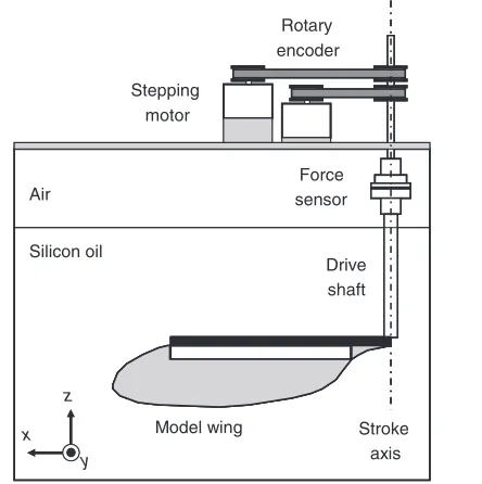
Fig.6 is a schematic diagram of the experimental apparatus of our dynamically scaled model. The computer-operated stepping motor rotates the drive shaft viathe timing belt and two pulleys to flap the model wing. The rotational angle of the drive shaft in one step is 0.35deg. The fluid forces acting on the model wing are measured by a force sensor, which is located in the drive shaft. We used a six-axis force and torque sensor (BL Autotec, Ltd, Kobe, Japan), which detects six components of forces and torques with six pairs of strain gauges affixed to a Y-shaped beam. From the calibration test using the loads of 10, 20, 30, …, 300gf, the force sensor revealed the force in the z-direction with an error of less than 1.3%. Note that the error is defined as the absolute error

divided by the maximum load 300gram-force, which

approximately corresponds to the maximum lift force in our experiment. The z-axis of the force sensor was set to be coaxial with the axis of the drive shaft. Thus, the z-axis of the force sensor was used to detect the lift FLgenerated by the wing flapping. The

precise flapping angle () was measured by a rotary encoder connected to the drive shaft viaa timing belt and two pulleys. The resolution of is 0.12deg. We used a high speed video camera (Citius Imaging, Ltd, Finland), which had a resolution of 640480 pixels and a sampling speed of 99framess–1_{, to record the whole} wing motion (camera viewpoints A and B in Fig.5). The pitch angle (q) was calculated using the chord length and its projection on the stroke plane given by the recording from viewpoint B, i.e. sine of the pitch angle qequals the projection divided by the chord length. We used a data acquisition system with a resolution of 16 bits and a sampling speed of 50,000sampless–1_{to collect the data} for and FLor and qat the same time. During data collection, we used a low-pass three-pole Butterworth filter with a cut-off frequency of 10Hz (implemented viaNI LabVIEW), roughly 20 times the flapping frequency, f. Each flight of the model wing consisted of eight continuous strokes. Five such flights were averaged for the same experimental condition. We used a silicon oil as the fluid. The x-, y- and z-dimensions of the oil filling the

Stroke angle _Φ

Upstroke

Downstroke Model wing

Camera

view point Camera

view point B

A z

x ϕ

y

Fig.5. Flapping motion of the model wing. The axes of the camera view points A and B are approximately coaxial with the x- and z-axes, respectively.

Table 1. Summary of the data for the crane fly reported by Ellington and Ennos

Individual mb (g) LW (cm) c (cm) rA mw (g) (deg.) f (Hz)

1/GI pr

[106 _{deg./(N m)]}

1/GI

sp

[106 _{deg./(N m)]}

CF01 CF02

1.9 10–2

1.14 10–2

1.37 1.27

2.62 10–1

2.32 10–1

10.5 10.9

1.48 10–4

1.13 10–4

123* 123

45.5* 45.5

62.3±24.9† 62.3±24.9†

449±244† 449±244† Average 1.52 10–2 _{1.32 2.47 10}–1 _{10.7 1.31 10}–4 _{123 45.5 62.3 449} *The valuesare taken from CF02.

†_{The valuesare taken from Ennos (Ennos, 1988a). The other data is taken from Ellington (Ellington, 1988a; Ellington, 1988b).}

mb, body mass; LW, longitudinal length of the wing (one wing); c, average wing chord length; rA, aspect ratio of the wing, 2Lw /c;mw, mass of wing; , stroke angle;f, flapping frequency;GIpr, torsional stiffness of the actual insect wing for pronation; , torGI sional sitffness of the actual insect wing for supination.

[image:4.612.46.568.81.132.2]

sp

Table 2. Values of the non-dimensional numbers for the crane flies derived using Eqn 3 and the averaged data in Table 1

Re St Chpr _Chsp _M

333 5.5510–2 _4.4910–3 _3.2410–2 _6.4210–2

Re, Reynolds number; St, Strouhal number; Chpr_{, Cauchy number for} pronation;Chsp_{, Cauchy number for supination;M, mass number.}

Force

sensor Rotary encoder

Stepping motor

Silicon oil

Model wing

Drive

shaft

Stroke

axis

z

x y Air

[image:4.612.315.568.210.239.2] [image:4.612.338.560.495.718.2] [image:4.612.50.280.503.707.2]

tank were 45, 75, and 33cm, respectively. The silicon oil had a density of f_{0.96gcm}–3_{and a dynamic viscosity of 0.5cm}2_s–1 (25°C). The wing longitudinal length (Lw), and the average chord length (c) were 22.5cm and 4.2cm, respectively, which satisfy the aspect ratio (rA) for the crane fly (see Table1). The stroke angle () was set to 123deg., which is equivalent to that for the crane fly (see Table1). The rigid beam used for the leading edge was made of stainless steel and had a cross section of 0.6cm0.6cm and length of 17.5cm. The rigid plate for the wing surface was made of polyethylene terephthalate (PET), with a thickness of 0.12cm. The flexible plate (plate spring) was made

of polyoxymethylene [POM; Young’s modulus: EFP2.59

1010_g/(cms2_{)], which had a thickness of t}

FP0.03cm or 0.05cm and a length in the chord direction of cFP1.0cm. The mass of the model wing, excluding the rigid beam, was mw10.7g.

Non-dimensional numbers of the proposed model

We determined the flapping frequency (f) and the wing longitudinal length of the flexible plate (lFP), such that the non-dimensional numbers for the proposed model were equivalent to those for the actual insect flight.

First, the Strouhal number (St) is considered. Eqn 3a can be reduced to St4/(rA). Thus, St is equivalent to that for the crane fly (St5.5510–2_{; see Table2) because and r}

A are equivalent to those for the crane fly.

Next, the Reynolds number (Re) is considered. Eqn 3b can be reduced to the following equation:

f2Re / (Lw c). (4) Using Eqn 4 and Re333 in Table2, the flapping frequency, f, is given as 0.52Hz.

7 cycles 7.5 cycles

7.125 cycles 7.625 cycles

7.25 cycles 7.75 cycles

7.375 cycles 7.875 cycles

Leading

edge Stroke axis

Plate spring

Wing surface

Next, the Cauchy number (Ch) is considered. Eqn 3c can be reduced to the following equation:

GM fVw,maxc4f/ Ch. (5) Using Eqn 5, ChChpr_{, Ch}A_{, C—h,Ch}B_{and Ch}sp_{, and Eqn 1, the} longitudinal length of the flexible plate lFPis given as 5.0cm for Chpr_{, 9.3cm for Ch}A_{, 6.0cm for C—h, 4.2cm for Ch}B_{and 3.3cm for} Chsp_{. Note that we used t}

FP0.05cm for the first lFPand tFP0.03cm for the rest.

Finally, the mass number (M) is considered. Using Eqn 3d, the mass number Mfor the proposed model is equal to 6.65, which is roughly 100 times larger than that for the crane fly (M6.4210–2_). It is difficult to satisfy the mass number condition since a solid material having a mass density 100 times larger than the present one is required to satisfy the mass number condition. A mass number roughly 100 times larger than that for the crane fly means that the inertial effect of the present model wing is roughly 1% of that of the actual insect wing (the reduced inertia of the model wing). However the dynamic similarity during the flapping translation was not much affected by the mass number since the inertial force during the flapping translation is not dominant because of the small acceleration. By contrast, the reduced inertia of our model wing would affect the wing rotation upon the stroke reversal where the acceleration is very large. In spite of this reduced inertia, however, the order of the rotational force might not be changed. The added mass during the stroke reversal is comparable to the wing mass in the insect flapping flight with the relative light wing (Bergou et al., 2007) and the added mass effect on our model wing is equivalent to that on the actual insect.

RESULTS AND DISCUSSION

Initially, the model wing was set to the position with a flapping angle of –/2 (see Fig.5, the upstroke is first). Then, after stabilizing at the static state, the up-stroke was started.

Passive pitching motion

Fig.7 shows sequences of snapshots of the motion of the proposed model wing in the case of ChC—hduring the seventh stroke using a high-speed video camera. Fig.8 shows the time history of the pitch angle (q) as well as that of the flapping angle (), the flapping angular velocity (d/dt), and the lift force (FL) in the case of ChC—h. The wing chord motion is shown in Fig.9, where the pitching motion was derived using the stroke and pitch angles from Fig.8A and C. These figures illustrate the typical flapping motion of our model wing during the whole of one stroke. Our model wing maintained a high angle of attack during the flapping translation and rotated quickly upon stroke reversal in all cases of Ch.

The model mid-stroke pitch angles were close to those of actual crane flies. The mid-stroke pitch angles are 27deg. for Chpr_{, 40deg.} for ChA_{, 49deg. for C—h, 54deg. forCh}B_{and 61deg. for Ch}sp_{, whereas} Ellington (Ellington, 1984b) reported the mid-stroke pitch angle for the actual crane fly are 45 or 55deg. during the downstroke and 55 or 65deg. during the upstroke at 70% of the wing length.

Fig.10 shows the relation between the Cauchy number and the mid-stroke pitch angle. The mid-stroke pitch angle has approximately linear dependency on the torsional stiffness. This result indicates that the present pitch angle during the flapping translation was maintained by the equilibrium between the elastic reaction force due to the wing torsion and the fluid dynamic pressure. As a consequence it is suggested that the equilibrium between the elastic reaction force and the aerodynamic pressure maintains a high angle of attack during the crane fly flapping translation.

The quick rotation of our model wing is surprising since the mass of our model wing provided only 1% inertial effect compared with the mass of the actual crane fly wing. This result would be explained by the added mass from the surrounding fluid. Recent study on the passive rotation using computational fluid dynamics (Bergou et al., 2007) has shown that the added mass during the stroke reversal is comparable to the wing mass for insects such as dragonflies and fruitflies, which have relatively light wings. Crane flies also have light wings, the weight of which is only a few percent of body weight. Note that the added mass effect on our model wing was equivalent to that on the actual crane fly wing because of the fluid dynamic similarity. Thus, the added mass might not change the order of the inertial force to rotate the wing upon the stroke reversal.

Lift force generated by the flapping wing with passive pitching

As shown in Fig.8C,D, the pitch angle, q, and the lift force, FL, covaried. It seems that they followed the kinematic characteristics of the flapping angle, , or the flapping angular velocity d/dt. Fig.11 shows the time histories of the lift force FLfor all Chas

A

B

–300 –150 0 150

300

d

ϕ

/d

t

(deg.

s

–1

)

ϕ

(deg.)

C

7.0 8.0

Cycles

Pitch

a

ngle (deg.)

D

–0.5 0 0.5 1.0 1.5 2.0

7.5 7.0 7.5 8.0

7.0 7.5 8.0 7.0 7.5 8.0

Lift (N)

–90 –60 –30 0

30 60 90

–90 –60 –30 0

30 60 90

Fig.8. Time histories of flapping angle (; A), flapping angular velocity (d/dt; B), pitch angle (q; C) and lift force (FL, D). We repeated the model wing flights five times. The FLdata for the individual flights (gray lines) and the average of the five flights (black line) are shown. d/dt was derived using the numerical time differential of .

Upstroke

Downstroke

well as the relation between Chand the mean lift coefficient (cL). The time histories of FLare similar to each other but their average values are different from each other. The average lift forces, FL, are 0.557N for Chpr_{, 0.753N for Ch}A_{, 0.772N for C—h, 0.746N forCh}B and 0.672N for Chsp_{. The corresponding lift coefficients C}

Lare 1.35, 1.83, 1.88, 1.81 and 1.63, respectively. These lift coefficients are close to those of the previous studies (Dickinson et al., 1999; Usherwood and Ellington, 2002b). The lift coefficients were calculated according to the following equations:

CL FL / [1/2 fAw (r2Vw)2], (6) where the fluid mass density f_{960kgm}–3_{(silicon oil, 25°C), the} area of the wing surfaceAw0.00945 m2given by cLw , the second moment of wing area r20.6 (Ellington, 1984a) and the mean wing tip velocity of the flapping motion Vw0.502ms–1given by 2fLw. The relation between Ch and the mean lift coefficient CL is

summarized in Fig.11F. It is interesting that the maximum CLwas achieved when C—h, which is the average of Chpr_{and Ch}sp_{, was used.} A mean lift coefficient (CLI) of 1.58 is required for the crane fly to hover if it is assumed that the insect can hover when the mean lift

FL(both wings) equals its body weight. The following parameters of the actual crane fly flight were used to calculate CLI: f1.205kgm–3 (air: 20°C), Aw3.2610–5m2, Vw2.58 ms–1and mb1.5210–5kg. The present CLfor ChA, C—h, ChBand Chspare larger than CLI, while the present CLfor Chpris slightly smaller than CLI. The translational lift would be well simulated in our experiment since, during the flapping translation, the dynamic similarity was not much affected by the inertial force because of the small acceleration. The rotational lift would be partly simulated because of the added mass effect from the surrounding fluid, but it would be weakened because of the reduced wing inertia. Evidence of the weakened rotational lift might be slight lift peaks observed before and after the stroke reversal (see Fig.11). The lift, which was composed mainly of translational lift, was sufficient to support the weight of the insect. This result is consistent with conventional studies of the aerodynamics of insect flight, i.e. the translational lift accounts for much of the lift required for the insect to hover while the rotational lift enhances the lift required for forward, upward accelerations or turn.

Our results suggest that the pitching motion in the actual crane fly flapping flight can be passive. Our purpose in this study has been achieved but the issue concerning the mass number still remains. We will address it in future work. We will also examine other dipterans to examine the applicability of our conclusion to their flapping flights.

APPENDIX

Non-dimensional numbers for the dynamic similarity between fluid–structure interaction systems

There are many non-dimensional numbers for the fluid–structure interaction (FSI) system, such as reduced velocity (Blevins, 1990;

0

30 60 90

0.04 0.02

0

Cauchy number

Pitch

a

ngle (deg.)

Fig.10. The relation between the Cauchy number and the mid-stroke pitch angle.

E

–0.5 0 0.5 1.0 1.5 2.0

8.0 7.5 7.0 6.0 6.5

Cycles

Lift (N)

C

–0.5 0 0.5 1.0 1.5 2.0

8.0 7.5 7.0 6.0 6.5

D

–0.5 0 0.5 1.0 1.5 2.0

8.0 7.5 7.0 6.0 6.5

A

–0.5 0 0.5 1.0 1.5 2.0

8.0 7.5 7.0 6.0 6.5

B

–0.5 0 0.5 1.0 1.5 2.0

8.0 7.5 7.0 6.0 6.5

Cycles

Lift (N)

F

1.0 1.3

1.5 1.8

2.0

0.04 0.03

Cauchy number

Me

a

n lift coefficient

0.02 0.01 0

Fig.11. Time histories of lift force (FL) for the cases of ChChpr_{0.0049 (A), ChCh}A_{0.0115 (B),}

Chakrabarti, 2002; Dowell, 1999), Cauchy number (Chakrabarti, 2002; Fung, 1956; Sedov, 1959), Stokes number (Paidoussis, 1998), mass number (Blevins, 1990; Dowell, 1999; Fung, 1956; Sedov, 1959) and reduced damping (Blevins, 1990), etc. We summarize here the equations governing the FSI system, the dimensional analyses for these equations and a set of the non-dimensional numbers used in the present study.

Equations governing fluid–structure interaction The body forces acting on the wing and the surrounding fluid are assumed to be zero. This assumption is justified by the fact that the gravitational force acting on the wing is only a few percent of the lift. Superscripts f and s denote fluid and solid quantities, respectively.

The fluid motion is described by the following Navier–Stokes equations for the incompressible viscous fluid:

where and viare the mass density and velocity, respectively, and

the stress tensor, ij, for a Newtonian fluid is:

where pand are the fluid pressure and viscosity, and ij is the Kronecker delta.

The wing motion is described by the following equation:

where d/dtin the left-hand side is the Lagrangian time derivative. The second Piola–Kirchhoff stress tensor for the linear isotropic Hookean elastic body is:

where and Gare the Lame constants and uiis the displacement.

The following equilibrium condition is satisfied on the fluid–structure interface:

f

ij· nfj+sij· nsj0, (A5)

where nf

jand nsjdenote the outward unit normal vectors for the fluid

and the structure, respectively.

Dimensional analyses for the governing equations We assume that the fluid and elastic body under the FSI share the following reference or characteristic quantities: length (L), displacement (U), velocity (V), pressure (Pf_V2_{) and time (T). In} terms of these common reference quantities, let us define the following non-dimensional variables:

xixi/ L, (A6a)

us

iuis/ U, (A6b) vs

ivsi/ V, (A6c)

vf

ivif/ V, (A6d)

pp / P, (A6e)

tt / T. (A6f)

ρf∂vif

∂t + ρfvfj

∂vif

∂xj =

∂σfji

∂xj

∂vif

∂xi =0 ,

, (A1a,b)

σijf = −pδij+ μ ∂vi

f

∂xj+

∂vfj ∂xi ⎛

⎝⎜

⎞

⎠⎟ , (A2)

ρsdvi

s

dt =

∂σsji

∂xj , (A3)

σijs= λδij∂uk

s

∂xk +G

∂uis

∂xj+

∂usj ∂xi ⎛

⎝⎜

⎞

⎠⎟ , (A4)

First, we apply dimensional analysis to the equation of the fluid motion (Eqn A1a) as described by Katz and Plotkin (Katz and Plotkin, 2001). Eqn A1a can be rewritten using the variables in Eqn A6 as:

Note that the term:

f_V2_{/ L (A8)}

in Eqn A7 represents the fluid inertial force due to the convective acceleration. Dividing Eqn A7 by Eqn A8 to obtain the non-dimensional form of Eqn A1a, as follows:

where

StL/ (TV), (A10a)

EuP/ (f_V2_{) 1, (A10b)}

and

Re f _{VL/ , (A10c)} are the Strouhal, Euler and Reynolds numbers, respectively.

Following the procedure similar to that for the fluid, we obtain the following form of the equation of motion for the elastic body, as follows:

Note that the term:

s_{V / T (A12)}

in the left-hand side of the above equation represents the magnitude of the structural inertial force due to the Lagrangian time derivative acceleration and that the coefficients of the two terms in the right-hand side represent the magnitude of the elastic force. Dividing Eqn A11 by Eqn A12 and using the relation UVT, we obtain the non-dimensional form of Eqn A3, as follows:

The coefficients of the first and second terms in the right-hand side of Eqn A13 are summarized using the relations 2G/(1–2) and E2G(1+) (is Poisson’s ratio, Eis Young’s modulus) as:

Rs sL2/ (ET2), (A14) which represents the ratio between the structural inertial force due to the Lagrangian time derivative acceleration and the elastic force. Finally, the non-dimensional numbers for the FSI are reduced as follows. Using the variables in Eqn A6, the fluid force f

ion the

fluid–structure interface can be rewritten as:

where Pand V/Lrepresent the fluid pressure and viscous force on the fluid–structure interface. Similarly, the elastic force s

ion the

fluid–structure interface can be rewritten as:

d ˆvis

d ˆt =

(λ +G)T2

ρsL2

∂2u_ˆ

k

s

∂xˆk∂xˆi+

GT2

ρsL2

∂2u_ˆ

is

∂xˆj∂xˆj . (A13)

ρsV

T d ˆvis

d ˆt =

(λ +G)U L2

∂2u_ˆ

ks ∂xˆk∂xˆi+

GU L2

∂2u_ˆ

is

∂xˆj∂xˆj . (A11)

St∂vˆif ∂_tˆ +vˆfj

∂vˆif

∂xˆj = −Eu

∂pˆ

∂xˆi+

1 Re

∂2_vˆ

if

∂xˆj2 , (A9)

ρf_V

T

∂vˆif

∂_tˆ +

ρf_V2

L vˆfj

∂vˆif

∂xˆj = −

P L

∂pˆ

∂xˆi+

μV

L2

∂2_vˆ

if

∂xˆ2j . (A7)

τif= σijf⋅nfj= −Ppˆ+μV

L

∂vˆif

∂xˆj+

∂vˆfj ∂xˆi ⎛

⎝⎜

⎞

⎠⎟nj

f _{, (A15)}

τis= σijs⋅nsj= λU

L

∂uˆ_ks

∂xˆk +

GU L

∂uˆis

∂xˆj+

∂uˆsj ∂xˆi ⎛

⎝⎜

⎞ ⎠⎟nj

Using the relations 2G/(1–2) and E2G(1+), U/Land GU/Lappearing in the right-hand side of Eqn A16 can be reduced to EU/L, which represents the elastic force on the fluid–structure interface. Dividing Eqn A15 by this term EU/L, two non-dimensional numbers for the non-non-dimensional form of Eqn A5 can be obtained. One is the ratio between the fluid dynamic pressure (Pf_V2_{) and the structural elastic force on the} fluid–structure interface (EU/L):

RPEP / (EU/L)  fVL / (TE). (A17) The other is the ratio between the fluid viscous (V/L) and elastic (EU/L) forces on the fluid–structure interface:

RVE / (EU/L)  / (TE), (A18) where the relation UVTis used. The ratio RPEhas the physical meaning equivalent to the Cauchy number Chf_V2_{/E(Chakrabarti,} 2002; Fung, 1956; Sedov, 1959) but it is the product of Ch multiplied by St. Instead of the usual expression, we use Eqn A17 as Chsince the FSI systems considered in the present study have a periodic input.

The other number for the FSI is the mass number (Blevins, 1990; Dowell, 1999; Fung, 1956; Sedov, 1959), which represents the ratio between the representative structural massmf_{and the fluid added} massms_:

M mf_{/ m}s_{ }f_L3_{/ m}s_{ }f_{/ }s_{, (A19)}

where the other expression of the representative mass, L3_{, is used} in the third and fourth expressions. Note that the fourth expression in Eqn A19 is equivalent to the ratio between the fluid inertial force due to the Eulerian time derivative acceleration (f_{V/Tin Eqn A7)} and the structural inertial force due to the Lagrangian time derivative acceleration (s_{V/T, Eqn A12).}

Non-dimensional numbers for the FSI system

The complete set of the non-dimensional numbers of the FSI system whose motion is described by the present governing equations are St, Re, Rs, M, RVEand Ch(RPE), which have the following two relations:

M St Re Rs RVE (A20a) and

Ch Re RVE. (A20b) We used the well-known numbers St, Re, Mand Chin the present study since the two relations (Eqn A20) make only four of St, Re, Rs, M, RVEand Chindependent.

LIST OF ABBREVIATIONS

q angular displacement around the wing longitudinal axis or the pitch angle

Aw the area of the wing surface

c average wing chord length

cFP flexible plate length in the chord direction

Ch Cauchy number

CL lift coefficient

EFP Young’s modulus of the flexible plate

f flapping frequency

FL total lift force acting on the wing GI torsional stiffness of the actual insect wing GM torsional stiffness of the model wing

lFP flexible plate length in the longitudinal direction (one wing) Lw longitudinal length of the wing (one wing)

mb body mass

mf added fluid mass

mw mass of wing

M mass number

Mq moment around the wing longitudinal axis

pr (superscript) pronation

rA aspect ratio of the wing, 2Lw /c

Re Reynolds number

sp (superscript) supination

St Strouhal number

tFP thickness of the flexible plate

Tw travel length of the leading edge center in the stroke plane V_w mean velocity of the flapping motion

Vw,max maximum speed of the flapping motion of the leading

edge center

f _{mass density of fluid}

 angular displacement of the flapping motion or flapping angle

stroke angle

This research was supported by a Grant-in-Aid from Japan Ministry of Education, Culture, Sports, Science and Technology. We would like to thank Professor M. Denda for the helpful discussion on the dynamic similarity law.

REFERENCES

Bergou, A. J., Xu, S. and Wang, Z. J.(2007). Passive wing pitch reversal in insect flight. J. Fluid Mech. 591, 321-337.

Birch, J. M. and Dickinson, M. H.(2003). The influence of wing-wake interactions on the production of aerodynamic forces in flapping flight. J. Exp. Biol. 206, 2257-2272.

Blevins, R. D.(1990). Flow-Induced Vibration. New York: Van Nostrand Reinhold. Chakrabarti, S.(2002). The Theory and Practice of Hydrodynamics and Vibration.

World Scientific Publishing Company.

Combes, S. A. and Daniel, T. L.(2003). Into thin air: contribution of aerodynamic and inertial-elastic forces to wing bending in the hawkmoth Manduca sexta. J. Exp. Biol. 206, 2999-3006.

Dickinson, M. H. and Gotz, K. G.(1993). Unsteady aerodynamic performance of model wings at low Reynolds numbers. J. Exp. Biol. 174, 45-64.

Dickinson, M. H., Lehmann, F.-O. and Gotz, K. G.(1993). The active control of wing rotation by Drosophila. J. Exp. Biol. 182, 173-189.

Dickinson, M. H., Lehmann, F.-O. and Sane, P. S.(1999). Wing rotation and the aerodynamic basis of insect flight. Science284, 1954-1960.

Dowell, E.(1999). A Modern Course in Aeroelasticity. Dordrecht, The Netherlands: Kluwer Academic Publisher.

Du, G. and Sun, M.(2008). Effects of unsteady deformation of flapping wing on its aerodynamic forces. Appl. Math. Mech.29, 731-743.

Ellington, C. P.(1984a). The aerodynamics of hovering insect flight. II. Morphological parameters. Phil. Trans. R. Soc. Lond. B 305, 17-40.

Ellington, C. P.(1984b). The aerodynamics of hovering insect flight. III. Kinematics. Phil. Trans. R. Soc. Londn B 305, 41-78.

Ellington, C. P., Van den Berg, C., Willmott, A. P. and Thomas, L. R.(1996). Leading-edge vortices in insect flight. Nature384, 626-630.

Ennos, A. R.(1987). A comparative study of the flight mechanism of Diptera. J. Exp. Biol. 127, 355-372.

Ennos, A. R.(1988a). The importance of torsion in the design of insect wings. J. Exp. Biol. 140, 137-160.

Ennos, A. R.(1988b). The inertial cause of wing rotation in Diptera. J. Exp. Biol. 140, 161-169.

Ennos, A. R.(1989). The kinematics and aerodynamics of the free flight of some Diptera.J. Exp. Biol. 142, 49-85.

Fung, Y. G.(1955). An Introduction to the Theory of Aeroelasticity. John Wiley & Sons, Inc.

Ishihara, D., Horie, T. and Denda, M.(2009). A two-dimensional computational study on the fluid-structure interaction cause of wing pitch changes in dipteran flapping flight. J. Exp. Biol. 212, 1-10.

Katz, J. and Plotkin, A.(2001). Low-Speed Aerodynamics. Cambridge University Press.

Liu, H., Ellington, C. P., Kawachi, K., Van den Berg, C. and Willmott, A. P.(1998). A computational fluid dynamic study of hawkmoth hovering. J. Exp. Biol. 201, 461-477.

Liu, Y. and Sun, M.(2008). Wing kinematics measurement and aerodynamics of hovering droneflies. J. Exp. Biol. 211, 2014-2025.

Miller, L. A. and Peskin, C. S.(2005). A computational fluid dynamics of ‘clap and fling’ in the smallest insects. J. Exp. Biol. 208, 195-212.

Paidoussis, M. P.(1998). Fluid-Structure Interactions: Slender Structures and Axial Flow. London: Academic Press.

Ramamurti, R. and Sandberg, W. C.(2002). A three-dimensional computational study of the aerodynamic mechanisms of insect flight. J. Exp. Biol. 205, 1507-1518. Sedov, L. I.(1959). Similarity and dimensional methods in mechanics. London:

Academic Press.

Sun, M. and Tang, J.(2002). Unsteady aerodynamic force generation by a model fruit fly wing in flapping motion.J. Exp. Biol. 205, 55-70.

Usherwood, J. R. and Ellington, C. P.(2002b). The aerodynamics of revolving wings II. Propeller force coefficients from mayfly to quail. J. Exp. Biol. 205, 1565-1576.

Vanella, M., Fitzgerald, T., Preidikman, S., Balaras, E. and Balachandran, B. (2009). Influence of flexibility on the aerodynamic performance of a hovering wing.J. Exp. Biol. 212, 95-105.

Walker, S. M., Thomas, A. L. R. and Taylor, G. K.(2009). Photogrammetric reconstruction of high-resolution surface topographies and deformable wing kinematics of tethered locusts and free-flying hoverflies. J. R. Soc. Interface6, 351-366. Wang, Z. J., Birch, J. M. and Dickinson, M. J.(2004). Unsteady forces and flows in