Munich Personal RePEc Archive
Does Financial Liberalization, Spur
Economic Growth and Poverty
Reduction in Six Sub-Saharan African
Countries; Panel Unit Root and Panel
Vector Error Correction Tests
Dandume, Muhammad Yusuf and A.C., Malarvizhi
Umaru Musa Yaradua University Katsina State-Nigeria, Multimedia
University Malaysia
February 2014
Online at
https://mpra.ub.uni-muenchen.de/52419/
Does Financial Liberalization Stimulate Economic Growth and
Reduce Poverty in Six Sub-Saharan African Countries?
Abstract
This paper examines the linkage among financial liberalization, economic growth and poverty reduction in
Sub-Saharan African countries (SSA). The study applies the recent panel Co-integration and vector error correction
mechanism to address the heterogeneity and cross-border interdependence over the period of 1980 to 2010. The
results reveal that economic growth is positively associated with poverty reduction and financial liberalization
coefficients are positively related to economic growth. It implies that financial liberalization causes economic
growth. However, the coefficients of financial liberalization are not significant in the poverty equation suggests that
financial liberalization does not have direct impact on poverty reduction in the six Sub-Saharan African countries.
This implies that the financial liberalization effects of poverty are upon contingent on the distributional changes
introduced by the growth and the configuration of institutions and policies that supported the liberalization process
and particularly, the existence or otherwise of good governance.
Key Words: Liberalization, poverty, economic growth, financial repression
1.0 Introduction
It is a well known the case that financial liberalization and its effects on economic growth and development has been
an area of considerable attention. Despite these prolific developments, little has been done on the relationship
between financial liberalization and reduction of poverty. The current bodies of literature have been, to a great extent
dominated by the free market neoclassical ideas which purported to show that financial sector liberalization
mobilizes savings and channels capital into the most appropriate product uses. By implication, both of which
improves the amount of physical capital and its productive uses. This invariably means, financial liberalization
raises the level of economic growth. By implication then, economic growth would raise the level of income and as
such reduce the level of poverty. Thus, with regards to countries in Sub-Saharan Africa these ideas have been
contested (Arestis and Glickman 2002). The recent development in most countries in Sub-Saharan Africa succinctly
raises a fundamental question of concern on whether financial liberalization exacts on both economic growth and
poverty reduction. Studies also question whether liberalization of the financial sector helps in the increase in the
amount of physical capital and productivity which could lead to economic growth and poverty reduction.
The revealing revelation about the SSA financial sector performance has indicated that the financial sectors of the
SSA countries are one of the poorly developed in the World. The average GDP per capita growth rate from 1961 to
2000 was 0.45percent. There is no much progress recorded in the mobilization of domestic resources for productive
proportion of GDP is below 20 percent. The financial global crisis accompanies financial liberalization has
worsened the internal resources to the region. On the social indicators, poverty and inequality of economic continue
to worsen indicating that economic growth has not been trickling down to the poor. The continent is experiencing a
jobless recovery from the financial meltdown, with a deteriorating fiscal deficit and current account balance. The
absolute number of people living in extreme poverty has been on the rise in SSA, the incidence of poverty fell
marginally, from 54 to 51 percent between 1981 and 2005 (UNDP, 2010). SSA faces major challenges in meeting
the 2015 Millennium Development Goal target. Furthermore, income inequality has grown in the region.
These associated characteristics of the SSA financial secotor performance raised the points of contestation whether
removal of all forms of restrictions on financial sector by allowing the market forces to allocate credit has created a
better performance of investments. Some studies have pointed out that most countries in Sub-Saharan African are
characterized by imperfect information, uncertainties, lack of perfect competitions, inadequate prudential
supervision coupled with a minimum level of accountability, poor legal framework and price instability (Arestis and
Glickman 2002). Therefore, it is questionable that liberalization of the financial sector based on the assumption of
perfect market can improve the level of physical capital and its productivity. From the perspective of mechanism,
some raised the question: what is the mechanism underlying the transition from financial repression to financial
liberalization to benefit various aspects of the society, especially for the poor? Despite, those questions, the
traditional free-market neoclassical economists supported by the IMF and World Bank still maintained the view that
the slow growth and the alarming rate of persistent poverty in Africa were attributed by financial repression. They
insist that the restriction on the financial transaction such as the interest rate control or considerable reserve
requirement causes slow growth and poor driven allocation of financial resources (Mckinnon, 1991).
On the general note, however, a more common view appears to be that whether financial liberalization lead higher
growth and poverty reduction or not in contingent on both domestic and external factors. Fry (1995) argued that
there is an urgent need for complementary effective prudential and supervision guideline with high level of
accountability, price stability and fiscal discipline Fry (1995) argument is that financial liberalization may not
increase the growth performance of the SSA countries since these countries are to some entend associated with
asymmetric information, lack of perfect competition, macroeconomic volatility as they are all manifest of market
failures. In such an environment, financial regulation may be the only choice to lower the interest rate in which the
average productivity by saving and investment can be stimulated. A lower interest rate could also, raise productivity
of physical capital through the low marginal cost of production and provide a venue of channeling pool saving into
technological deficiencies sectors. The general agreement is that financial liberalization depends upon the
institutional context of the economy of the SSA and, particularly the prevalence of good governance or otherwise.
This also raised the issue of whether the increased growth due to liberalization is supported by equitable income
distribution that allow poor people to share in growth (Arestis 2005).
The objectives of this paper are to empirically examine the preposition purports to show that six SSA countries
(Nigeria, Ghana, Cote D'Ivoire, Cameroun, Gambia, Botswana that liberalized their financial sector tend to grow
and Ndikumana, 2000 and Aziakpomo, 2004) have employed Panel GMM but the problem with their panel time
series analysis they often assume slope homogeneity or cross-sectional independence, which may lead to incorrect
causal inferences. This study aims to improve often on the previous studies in the SSA region by Panel
co-integration and Panel Causality which provide sample heterogeneity and examine the cross- country
interdependence. Utilizing both time-series and cross-sectional data from seven SSA countries over the period of
1980 to 2010.
The remaining part of this study is structured as follows: The subsequent part of the paper reviews the theoretical
and empirical literatures connecting financial liberalization to growth and poverty reduction. Section 3 presents
methods and materials of the study while section 4 presents the results and discussions. Finally section 5 ends the
paper with a summary and conclusions.
2.0 Materials Studied
2.1 Theoretical literature
The relationship between financial sector liberalization and economic development could be linked to contrasting
perspectives of finance and growth theories, each promoting different ways of influence. These differences have led
to a number of empirical researches to test the reliability of these approaches; hence different conclusions were
derived from the studies.
There are two major schools of thought advancing the argument on financial liberalization which includes the
finance-based theory or interventionists and neoclassical free market advocates, each advocating different
transmission mechanism of the linkage between the financial sector, economic growth and poverty reduction.
According to the non-interventionists theories which was associated with the work of Mckinnon and Shaw (1973)
which were built on the work of Schempeter (1911) provides two important ways in which financial repression
affects economic growth. The first, they believed that financial repression affects the efficiency of saving allocation
and the productive investment, in other words, financial repressions affect the rate of return on saving and even
affect the equilibrium level of saving and investment. This happened because investment is affected by the decision
of bankers who allocate investment funds according to their discretion, without considering the marginal
productivity of investment. These tendencies from the banker’s decision in turn, discourage the potential savers and
persuade them to keep their savings in unproductive assets. Secondly, excessive increase in the level of reserve
requirement decreases the supply of cash to the banks hence, affects their lending, and credit allocation.
To ameliorate these problems, this school of thought suggests systematic elimination of regulatory control measures
and operational guidelines, such as removal of the credit control program, deregulation of interest rate ceilings and
decreasing the reserve requirements, which will in turn stimulate economic growth and efficient allocation of
regulating the financial sector was the major cause of the declined in the real rate of growth and the real rate of the
financial development in relation to the non financial sectors. Such as removing all forms of restriction on the
interest rate and allow it to be determined by the free- market equilibrium level, will enhance the level of both
savings and productive investment.
On the contrary, the interventionists/ financial regulation theorists lunched their criticism on the financial
liberalization thesis based on the Keynesian model which emphasized on the role of effective demand. According to
the interventionists’ views, a shift in the deposit interest rate raises the marginal propensity to save and as such
decreases aggregate demand. A fall in aggregate demand and output causes a fall in profit and fall in profit causes a
fall in investment. This means that investment will be lower under financial liberalization than that in the financial
repression (Stiglizt 2000). The second criticism of the financial liberalization thesis emerged from the work of
Stiglitz, (1999); Fry, (1995); Arestis and Demetriades (1999) holds the believed that financial liberalization is prone
to market failure because of high information costs which is associated with high transaction costs. This is due to
the facts that monitoring banks are part and parcel of public goods therefore, high information costs create negative
externalities which have multiplier effects on the entire rest of the economy.
However, those views where an attack to the early growth theory of Slow (1952) who stresses the importance of
capital accumulation and sufficient saving for achieving faster economic growth and more efficient allocation of
resources through free market fundamentals.
On the empirical grounds, findings on the relationship between financial liberalization and growth, however, are
mixed and inconclusive. The general agreement is that higher level of financial sector development is associated
with high rates of economic growth, while some argue against. One of the interesting works in support of this
hypothesis is the work of Bonfiglioli (2008) who use dynamic panel analysis based on the system GMM on the
variables of liberalization, growth and poverty, drawing data from samples of selected countries out of 70
developing and developed countries. The results revealed that financial liberalization significantly impact on
productivity growth. However, the problems with the study of Bonfiglioli (2008) are presumed slope homogeneity
without taking into cognizance the heterogeneity in the sample size.
Gehringer et al (2013) examines the causal linkage between financial sector reforms and economic growth, drawing
data from 26 EU countries, between 1990- 2007; using the techniques of difference GMM. Their findings revealed
that financial integration has significant positive impact on economic growth among the EU countries. Another
multinational study is associated with the work of Bonfigioli (2008b) who examine the impact of financial
liberalization on growth performance. Taking samples of 28 manufacturing industries from 56 countries over the
period of 1963-2003. The results of the study indicated that financial liberalization positively affects economic
growth along with entry of firms, capital accumulation and raised the level of employment. Another study of
Bonfiglioli et al (2011) examines the linkage between financial liberalization and factor productivity and capital
accumulation, using data of 96 countries collected between 1998-2006, employing the techniques of pooled OLS.
Fowowo (2013) examine financial sector reforms and the productivity in private investment in SSA, using a
developed index. He applied the techniques of generalized method GMM in order to address the problem of
endogeneity bias. The study confirmed that financial sector reforms have had positive effects on private investment
in the selected Sub-Saharan Countries. But the problem with the study is the application of GMM which assume
slope homogeneity without capturing coefficients heterogeneity and cross- sectional interdependence.
On the contrary, the findings of other studies have provided disappointing results of financial liberalization on
economic growth. Such as the study of Stiglizt (2000) whose findings revealed that financial liberalization does not
actually address the problems of asymmetric information which affects the intimidation function of a liberalized
market existing in the poor countries.
Enowbi Batu (2012) use different approaches to measure financial liberalization and banking crisis. The findings of
the study suggested that even though liberalization may succeeds in reducing the cost of production but there is the
possibilities that banks may end up financing more risky projects and over time project with lower return will be
accepted which could make banks more vulnerable to crisis. Oshikoya (1992) apply time-series data to measure the
effects of interest rate liberalization on economic growth in Kenya uses the data of 1970 to 1989. The findings of the
study indicate that liberalization of interest rate causes economic growth in Kenya.
Soyibo and Ade (1994) use the method of correlation graphs to measure the linkage between economic growth and
financial intermediation, collected data from 11 countries in Africa, using the ratio of currency, demand deposits,
and time and saving deposits to GDP. The results of their study did not show any evidence that financial
liberalization causes economic growth.
The debate on the linkage between financial liberalization and poverty has little attention in the academic research.
Some of the claims both at theoretical and empirical level have been mixed. One of the noteworthy study, is the
work of (Jalilian and Kirkpatricks, 2002) who examine the nexus between financial liberalization and poverty via
economic growth. These authors' study was motivated by the work of Dollar and Kraay whom study confirms the
positive impact of economic growth on poverty. The authors estimate two equations, a growth and poverty
regression in the growth regression; they pay more attention on the financial liberalization variables in the
estimation. The authors also identified a number of control variables in the poverty regression. The finding of their
study indicates that one unit change in financial liberalization is associated with a 0.4 percent change in the growth
rate of the income of the poor.
Another study associated with the work of Ariste, et al (2004), provides way through which financial liberalization
affects poverty. One of such ways is through financial crisis which follow after financial liberalization of which lead
to fall in the earnings of both the formal and informal-sector workers due to job losses in the formal sector and fall
in the demand for services in the informal sector.
Fowowo (2011) argue that the poor are denied access to institutional finance because financial liberalization fails to
linkages between financial institutions and poverty reduction argued that financial development affect only one
segment of the society whose shares of income is under one dollar a day. In a related study Beck et al (2008) apply
cross-sectional analysis of 52 developing and developed countries over a period of 1960 to 1990. They found that
financial intermediary development has a significant impact on the poor. Thus, the critiques note, the problems with
the study of Honohan (2004) and Beck et al (2008) is the omission of variable biases.
However, in order to address the methodological problems with the studies of (Honohan, 2004; Beck et al , 2008).
Jeanneney and Kpodar (2011) integrated the variable of financial instability into financial development variables.
The results of their study indicate that financial depth,? Is significantly affecting poverty reduction. But they argued
that the ratio of credit to GDP did not positively affect poverty reduction. They used econometric analysis as an
evidence to support Mckinnon (1973) views that financial intermediaries do not directly affects poverty reduction
but have a great influence on economic growth which in turn affect poverty reduction indirectly.
Whether financial liberalization leads to better access to credit for the disadvantage borrowers and savers, the study
of Len Sink (1996) provides indebt explanation. The author argued that financial liberalization through the formal
sector may cause decreases in savings and decreases in the amount of investment which results in the decline in the
allocative efficiency of capital. The author argues that in SSA financial liberalization failed to realize that the formal
banking sector are less important for financing investment project.
3.0 Methods
To examine the relationship between financial liberalization, growth performance and reduction in poverty this
study used the data collected from six countries over the period 1996 to 2011. Growth of real GDP per- capita (real
GDP per capita in constant price) was used to measure economic growth. We use poverty represented by the head
counts index (defined as the percentage of the population under a dollar daily income) Data were extracted from the
WDI (World Bank). Chin- Ito index were used to represent financial openness. These indexes allowed to investigate
the extent of financial openness for a country in a given period of time, which was developed based on binary series
based on the IMF report of exchange Arrangement and exchange restriction (AREAR). The rest of the indices
(FR1andFR2) are developed from five component parts of the financial liberalization policies
The common problems with previous studies on panel time series analysis they often assume slope homogeneity or
cross-sectional independence, which may lead to incorrect causal inferences. This study aims to improve often on
the previous studies in the SSA region by using Panel co-integration and Panel Causality which provide sample
heterogeneity and examine the cross- country interdependence. In this case co-integrating vectors are used through
the fully modified (FM) OLS approach which take care of the heterogeneity of the coefficients and also allow
consistency in the long run relationship with the short- run adjustment. The countries studied are Nigeria, Cameroun
Ghana, Gambia, Botswana and Cote D'Ivoire.
Different approaches for the estimation of a unit root in a panel data has been established with the aim of integrating
information from time series data with that of the cross-sectional information. These are classified under the four
panel unit root test which is Levin, Lin and Chu (LLC) test, IM, Pesaran and Shin (IPS) test and PP- fisher test. The
first generation test was developed by Levin and Lin (1993) which suffer a number of shortcomings. The problem
with this first generation test is that they do not allow for heterogeneity in the autoregressive coefficient. This new
generation test was specified as follows:
, t
i
,
,
(1)
i
t
ij
i t
j
i t
β
ϕ
β
ϕ
β
η
∆
=
+
+
∑
∆
− +
− − −
Where
∆
the first difference operation ηi is the random terms and sigma for changes ofφ2
,
1, 2
t
=
− −
T
stand for
time period, and
1, 2
10
i
=
− − −
represents regional cross- time series
This approach made it easy to determine the two dimensional fixed effects (
δ
and
∂
) and unit exact period time
trends. Levin, Lin and Chu test, includes the first and null hypothesis
:
0
Ho
β =
i
for all i, which is tested on the
opposite under the alternative hypothesis
0
Hi i
β
=
β
p
for all i.
However, the framework, of analysis was extended by the Levin, Lin and Chu (2002) analysis in order to take care
the presence of heterogeneity of the coefficient terms in the alternative hypothesis. While on the other hand, Pesaran
and Shin (2003) have compromised the similarity of the first order AR coefficient of the Levin, Lin and Chu test that
enable
β
become not similar along the cross-sectional region in the alternative hypothesis. Both hypotheses are
specified as H0;
i
β
=0 ˂ i, HI=
i
β
˂ 0 in certain i. While IPS measure is conducted on the basis of the mean group
procedure IPS exhibit their approach as appropriate with the finite sample ability when compared with the Levin Lin
and Chu approach. The Fisher-ADF test developed by Choi (2001) and the Fisher, PP test developed by Pedroni
(1999) used probability by applying an asymptotic Chi-Square approach. One good merit of using the Fisher test, in
place of IM Pesaran test, it doesn’t need balance panel, it also enable the application of various lag lengths in the
separate ADF estimate and can be easily estimated in the case of any derived Unit roots test. The major demerit of
the Fisher test lies in the way the Probability- values were established based on Monte Carlo.
Pedroni (1999) developed various estimates using residuals found in the work of the Engle and Granger, (1987)
Panel co -integration techniques allow the estimation of homogeneity. Because heterogeneous parameters, fixed
effects and individual specific deterministic trend are all allowed Pedroni (2004). With this development Pedroni
established Seven Panel co- integration statistics, four are known as the pool panel co- integration statistics, and they
are categorized within dimension based statistics. While the rest of the three are called mean panel co- integration
statistics and they all fall between-dimension based.
Pedroni (1999) pointed out that long time period cases with a number of observations above 100 have a minimum
sample size distortion, thereby maintaining a large power of test within the seven statistics in all cases. On the
contrary panel with short spans their alternative statistics yield conflicting results. Engle and Granger (1987)
pointed out that the group of ADF reveals a better testing power, followed by Panel ADF. But on the other hand, the
panel-variance and group p statistics function less effectively in relative to the others.
Panel Vector Error Correction Model
Whenever, a model is found to be co-integrated it indicates the possible existence of causality which is determined
through the application of PVECM
,
,
1
,
(2)
it
Ci
k
i t
k
teci t
Ui t
δ
β
δ
λ
∆
=
+ ∑
∆
− +
− +
− − −
Where
δ
is the vector of variables, comprising the GDP, POVT, KO, and FR1and FR2.While “I” stand for Panel
characteristics of cross-country analysis, “ec” stands for the error terms λ ui stand for the rate of adjustment to the
long run equilibrium equally.
4.0 Results and Discussions
Before proceeding to integration and causality test it is imperative to provide the descriptive analysis of the data to
ensure whether the data is normally distributed or otherwise. In a situation where the data appear with certain
abnormalities the integration order to the data has to be ensure in all series. In doing so we estimated the descriptive
statistics in table 1 below as well as the unit root test in both level and first difference and the results are presented in
[image:9.612.72.535.612.740.2]tables 2 and 3 below.
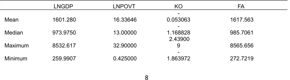
Table 1 descriptive statistics
LNGDP LNPOVT KO FA
Mean 1601.280 16.33646
-0.053063 1617.563
Median 973.9750 13.00000
-1.168828 985.7061
Maximum 8532.617 32.90000
2.43900
9 8565.656
Minimum 259.9907 0.425000
Std. Dev. 1719.814 10.62194
1.54931
6 1724.730
Skewness 2.202836 0.128556
0.81406
5 2.207758
Kurtosis 7.356604 1.861378 1.851194 7.361976
Jarque-Bera 153.5597 5.450261
15.8822
5 154.0945
Probability 0.000000 0.065538
0.00035
6 0.000000
Sum 153722.9 1568.300
-5.094045 155286.1
Sum Sq.
Dev. 2.81E+08 10718.43
228.036
0 2.83E+08
Observation
[image:10.612.75.529.75.297.2]s 96 96 96 96
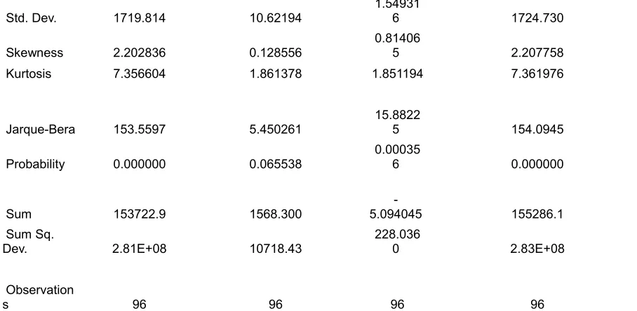
[image:10.612.68.551.413.519.2]Table 1 above indicate that skewness is not closed to zero on LNGDP and FA, while in the case of LNPOVT and KO skewness is achieved. Thus Kurtosis is not closed to three on LNPOVT and KO and it is greater than three in the LNGDP and FA. This indicate that the data is not normally distributed. However the probability also reveals that the data is not greater than 5 percent as such the data is not normally distributed. This call for the unit root test in order to ensure that the data is cointegrated before its application into estimation.
Table 2 panel unit root results at level
LL IPS ADF-Fisher Pp-fisher
FA -1.27516 (0.1011) -0.58884 (0.2780) 12.7764 (0.3855) 14.2748 (0.2835) LPOVT -2.29915 (0.0107) 2.35794* (0.0092) 17.7229 (0.0234) 19.2979 (0.0133) LNGDP -0.06881 (0.4726) -0.31575 (0.3761) 21.1638 (0.0200) 37.8803* (0.0000) KO -1.46401 (0.0716) -1.12256 (0.1308) 19.0032 (0.0885) 22.0047 (0.0376) Note: * ** and *** suggest the rejection level at the 10%, 5% and 1% level accordingly.
Table 2
presents the results of the panel unit root test with LLC, IPS, ADF, Fisher and PP- fisher
test.
The results of the null unit root test at level indicate that the series are not stationary at level with the exceptionof LPOVT which is significant at IPS and LNDGDP at PP fisher. In order to ensure the stationary of the data another
Table 3 panel Unit root results at first difference
LCC IPS ADF-Fisher PP-Fisher
FA -12.6132* (0.0000) -11.1293* (0.0000) 113.416* (0.0000) 127.088* (0.0000) LPOVT -8.52930* (0.0000) -8.21637* (0.0000) 59.0147* (0.0000) 59.0076* (0.0000) LNGDP -7.62512* (0.0000) -6.27426* (0.0000) 77.9587* (0.0000) 97.3907* (0.0000) KO -12.6504* (0.0000) -11.5028* (0.0000) 116.041* (0.00000) 143.2144* (0.00000) Note: * ** and *** suggest the rejection level at the 5%, 10% and 1% level accordingly.
Table 3 present the results of the panel unit root test with LLC, IPS,ADF, Fisher and PP- fisher test. The results
indicates that all series become stationary after first difference, at 5% level of significance, therefore, the null
hypothesis that there is unit root is rejected at first differences. With these the data is suitable for the econometrics
[image:11.612.65.556.451.547.2]estimation and anaylsis.
Table 4 panel Co-integration test results (poverty as a dependent variable)
Statistics P-value
Panel V -1.204393 0.8867
Panel P 1.124252 0.8867
Panel PP 1.019771* 0.0067
Group ADF 1.663833 0.9519
Group P -0.869024 0.1924
Group PP -4.85135* 0.0000
Group ADF -11.7663* 0.0000
Note: * ** and *** suggest the rejection level at the 5%, 10% and 1% level accordingly.
To examine whether the variables under investigation
Table 4 is estimated to determine whether there is co- integration relationship among LNGDP KO, FA and LPOVT
in SSA, through the newly established approach to panel co-integration developed by Pedroni (2004). The approach
involves four panel statistics and three group panel statistics.
The results indicate that the null hypothesis of no co integration is rejected at 5% level of significance on panel PP,
Group PP and Group ADF test statistics. This indicates that the variables move together towards stable equilibrium
poverty reduction in SSA. However, having long run relationship does not mean causality, as such to determine the
[image:12.612.70.541.188.358.2]direction of the causality, we estimate and analyse causality in the table 4
Table 5 panel vector error correction mechanism results
Independent Var. ∆LPOVTt ∆LNGDPt ∆KO ∆FAt
ECt-1 1.483692*
(-2.62323) 0.122430* (-3.46582) 0.0206598* (-2.95300) 0.059365* (-1.99367)
∆LPOVTt-1 0.147188
(0.64967) -7027661 (-0.26426) 0.001401 (0.12120) 0.001025 (0.50103)
∆LNGDPt-1 1.009466*
(2.21335) -0.059555 (-0.75445) -8951112 (-0.26087) 2.599912 (0.43168)
∆KOt-1 -0.257390
(0.07723) 1.170008* (2.45892) -0.229702 (-2.81355)
---∆FAt-1 0.844202
(0.26263) 6.766608* (2.65196) --- -0.087920 (-1.10743) C 0.273772 (-0.24891) -1.8670902 (-0.17813) -7.566605 (-0.00166) -9.233305 (-0.01166)
Note:*** ** and * indicate the significance at the 5%, 10%, and 1% accordingly. The P- Value is given in
parentheses.
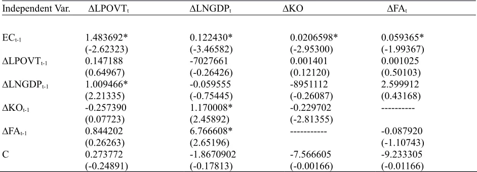
The results in table 5 above indicate that the error correction term is statistically significant with a positive
coefficient on poverty model, suggesting that past disequilibrium changes in the poverty will be adjusted back to the
steady and stable equilibrium in the current period. Hoever, in the poverty model with ∆LPOVTt as the dependent
variable the econometric result of the investigated coefficient of ∆LNGDPt-1 indicates a statistically significant
positive value. This suggests that economic growth contributes to poverty reduction. . Additionally, the coefficients
of ∆KOt-1 and ∆FAt-1 which are the proxies of financial liberalization are significantly positive implying that
financial liberalization has impacts on economic growth
However, the coefficients of ∆KOt-1 and ∆FAt-1 which are the proxies of financial liberalization are not significant,
suggesting that financial liberalization does not have direct impact on poverty reduction. Thus, the six Sub-Saharan
African country's financial liberalization does not have a direct impact on poverty reduction. The policy implication
is that financial liberalization required an intervention policies which focus on the poor. Other wise certain group of
few individuals may continue enjoying the benefit of financial liberalization at the expense of the poor.
In recent years many countries in SSA have witnessed tremendous reforms of their financial sector. While studies on
the financial sector reforms and its benefit on economic growth and poverty reduction has received a great deal of
attention. ( Mckinnon and Shaw 1973), This study investigates the causal linkage among the liberalization policy of
the financial sector, economic growth and poverty reduction implemented within six SSA, This study contributes by
utilizing financial liberalization indices that adequately capture the gradual nature and intensity of the financial
market reforms. The study employed the techniques of panel Co integration and panel vector error correction
mechanism in addressing the common mistake found in the previous studies of assuming slope homogeneity and
cross-sectional interdependence.
The econometric results reveal that even though financial liberalization impact on economic growth, but the
assumption that financial liberalization will at the end impact the poor through trickle down effects is not always the
case. In the case of SSA the findings have shown that financial liberalization without first, sustaining
macroeconomic stability, regulatory and supervisory frameworks, sound institutions and policies the financial sector
liberalization may end up worsening the living standard of the poor. The implication is that financial liberalization in
the case of SSA needs to be fashion out with poverty reduction thrust in order for the program to benefit the poor
segment of the society.
Reference
Arestis, P., and Demetriades, P. (1999). Financial liberalization: the experience of developing countries. Eastern
Economic Journal, 25(4), 441-457.
Arestis, P., and Stein, H. (2005). An institutional perspective to finance and development as an alternative financial
liberalisation. International Review of Applied Economics, 19(4), 381-398. http://www.levyinstitute.org/pubs/wp377
Beck, T., and Levine, R. (2008). Legal institutions and financial development: Springer. http://www.nber.org/papers
Bencivenga, V. R., & Smith, B. D. (1991). Financial intermediation and endogenous growth. The Review of
Economic Studies, 58(2), 195-209.
Bonfiglioli, A. (2008). Financial integration, productivity and capital accumulation. Journal of International
Economics, 76(2), 337-355. doi:10.1016/j.jinteco.2008.08.001
Chinn, M., and Ito, H. (2011). Financial Globalization and China. forthcoming in the Encyclopedia of Financial
Globalization, edited by Gerard Caprio, et al.(Elsevier).
Practice: Frontiers of Analysis and Applied Research: Essays in Honor of Peter CB Phillips. Cambridge University Press, Chapt, 11, 311-333.
Enowbi Batuo, M., and Mlambo, K. (2012). Financial liberalisation, Banking Crises and Economic Growth in
African Countries. http://mpra.ub.uni-muenchen.de/id/eprint/41524
Fowowe, B. (2008). Financial Liberalization Policies and Economic Growth: Panel Data Evidence from
Sub‐Saharan Africa. African Development Review, 20(3), 549-574. DOI: 10.1111/j.1467-8268.2008.00198.x
Fowowe, B. (2013). Do Fiscal Incentives Promote Investment?: Empirical Evidence from Nigeria. The Journal of
Developing Areas, 47(2), 17-35. DOI: 10.1353/jda.2013.0029
Fry, M. J. (1997). In favour of financial liberalisation*. The Economic Journal, 107(442), 754-770.
Green, H. J. (1960). Growth models, capital and stability. The Economic Journal, 57-73.
Honohan, P. (2004). Financial development, growth, and poverty: how close are the links? : World Bank.
wds.worldbank.org/servlet/WDSContentServer/WDSP/IB/2004/03/30/000160016_20040330143253/Rendered/PDF
/wps3203.pdf
Im, K. S., Pesaran, M. H., and Shin, Y. (2003). Testing for unit roots in heterogeneous panels. Journal of
Econometrics, 115(1), 53-74.
Iyengar, B., Gehringer, E., Wolf, M., & Manivannan, K. (2013). Scalable concurrent and parallel mark. ACM
SIGPLAN Notices, 47(11), 61-72.
Jeanneney, S. G., and Kpodar, K. (2011). Financial development and poverty reduction: Can there be a benefit
without a cost? The Journal of Development Studies, 47(1), 143-163.
King, R. G., and Levine, R. (1993). Finance and growth: Schumpeter might be right. The quarterly journal of
economics, 108(3), 717-737.
Levin, A., Lin, C.-F., & James Chu, C.-S. (2002). Unit root tests in panel data: asymptotic and finite-sample
properties. Journal of Econometrics, 108(1), 1-24.
McKinnon, R. I. (1989). Financial liberalization and economic development: a reassessment of interest-rate policies
McKinnon, R. I. (1991). Financial control in the transition from classical socialism to a market economy. The Journal of Economic Perspectives, 5(4), 107-122.
Oshikoya, T. W. (1992). Interest rate liberalization, savings, investment and growth: the case of kenya/liberalisation
des taux d'interet, epargne, investissement et croissance: le cas du kenya. Savings and Development, 305-32
Pedroni, P. (2004). Panel cointegration: asymptotic and finite sample properties of pooled time series tests with an
application to the PPP hypothesis. Econometric theory, 597-625.
Soyibo, A. (1994). Characteristics of the savings-investment process in Nigeria. World Development, 22(8), 119
1210.
Stiglitz, J. (1999). Whither reform. Washington DC: The World Bank.