Optimization and Sampling for NLP from a Unified Viewpoint

Optimization and Sampling for NLP from a Unified Viewpoint

Marc DYMETMAN

_{Guillaume BOUCHARD}

_{Simon CARTER}

(1) Xerox Research Centre Europe, Grenoble, France (2) ISLA, University of Amsterdam, The Netherlands

{marc.dymetman,guillaume.bouchard}@xrce.xerox.com; [email protected]

Abstract

The OS* algorithm is a unified approach to exact optimization and sampling, based on incremental refinements of a functional upper bound, which combines ideas of adaptive rejection sampling and of A* optimization search. We first give a detailed description of OS*. We then explain how it can be applied to several NLP tasks, giving more details on two such applications: (i) decoding and sampling with a high-order HMM, and (ii) decoding and sampling with the intersection of a PCFG and a high-order LM.

1 Introduction

Optimization and Sampling are usually seen as two completely separate tasks. However, in NLP and many other domains, the primary objects of interest are often probability distributions over discrete or continuous spaces, for which both aspects are natural: in optimization, we are looking for the mode of the distribution, in sampling we would like to produce a statistically representative set of objects from the distribution. The OS∗_{algorithm approaches the two} aspects from a unified viewpoint; it is a joint exact Optimization and Sampling algorithm that is inspired both by rejection sampling and by classical A∗_{optimization (O S}∗_).

Common algorithms for sampling high-dimensional distributions are based on MCMC techniques

[Andrieu et al., 2003, Robert and Casella, 2004], which are approximate in the sense that they

produce valid samples only asymptotically. By contrast, the elementary technique of Rejection Sampling[Robert and Casella, 2004]directly produces exact samples, but, if applied naively to high-dimensional spaces, typically requires unacceptable time before producing a first sample. By contrast, OS∗_{can be applied to high-dimensional spaces. The main idea is to upper-bound} the complex target distributionpby a simpler proposal distributionq, such that a dynamic programming (or another low-complexity) method can be applied toqin order to efficiently sample or maximize from it. In the case of sampling, rejection sampling is then applied toq, and on a reject at pointx,qis refined into a slightly more complexq0_{in an adaptive way. This} is done by using the evidence of the reject atx, which implies a gap betweenq(x)andp(x), to identify a (soft) constraint implicit inpwhich is not accounted for byq. This constraint is then integrated intoqto obtainq0_.

is already unlikely at the bigram level: the bigram constraints present in the proposalqwill ensure that this sequence will never (or very rarely) be explored byq.

The case of optimization is treated in exactly the same way as sampling. Formally, this consists in moving from assessing proposals in terms of theL₁norm to assessing them in terms of the

L_∞norm. Typically, when a dynamic programming procedure is available for sampling (L1 norm) withq, it is also available for maximizing fromq(L_∞norm), and the main difference between the two cases is then in the criteria for selecting among possible refinements. Related work In order to improve the acceptance rate of rejection sampling, one has to lower the proposalqcurve as much as possible while keeping it above thepcurve. In order to do that, some authors[Gilks and Wild, 1992, Görür and Teh, 2008], have proposedAdaptive Rejection

Sampling (ARS)where, based on rejections, theqcurve is updated to a lower curveq0_with

a better acceptance rate. These techniques have predominantly been applied to continuous distributions on the one-dimensional real line, where convexity assumptions on the target distribution can be exploited to progressively approximate it tighter and tighter through upper bounds consisting of piecewise linear envelopes. These sampling techniques have not been connected to optimization.

One can find a larger amount of related work in the optimization domain. In an heuristic optimization context the two interesting, but apparently little known, papers[Kam and Kopec, 1996, Popat et al., 2000], discuss a technique for decoding images based on high-order language

models where upper-bounds are constructed in terms of simpler variable-order models. Our application of OS∗_{in section 3.1 to the problem of maximizing a high-order HMM is similar to} their (also exact) technique; while this work seems to be the closest to ours, the authors do not attempt to generalize their approach to other optimization problems amenable to dynamic programming. Among NLP applications,[Kaji et al., 2010, Huang et al., 2012]are another recent approach to exact optimization for sequence labelling that also has connections to our experiments in section 3.1, but differs in particular by using a less flexible refinement scheme than our variable-order n-grams. In the NLP community again, there is currently a lot of interest for optimization methods that fall in the general category of “coarse-to-fine" techniques[Petrov, 2009], which tries to guide the inference process towards promising regions that get incrementally tighter and tighter. While most of this line of research concentrates on approximate optimization, some related approaches aim at finding an exact optimum. Thus,[Tromble and Eisner, 2006]attempt to maximize a certain objective while respecting complex hard constraints, which they do by incrementally adding those constraints that are violated by the current optimum, using finite-state techniques. [Riedel and Clarke, 2006]

have a similar goal, but address it by incrementally adding ILP (Integer Linear Programming) constraints. Linear Programming techniques are also involved in the recent applications of Dual Decomposition to NLP[Rush et al., 2010, Rush and Collins, 2011], which can be applied to

difficult combinations of easy problems, and often are able to find an exact optimum. None of these optimization papers, to our knowledge, attempts to extend these techniques to sampling, in contrast to what we do.

Paper organization The remainder of this paper is structured as follows. In section 2, we describe the OS∗_{algorithm, explain how it can be used for exact optimization and sampling,} and show its connection to A∗_{. In section 3, we first describe several NLP applications of the} algorithm, then give more details on two such applications. The first one is an application to optimization/sampling with high-order HMMs, where we also provide experimental results;

optimiza-tion/sampling with the intersection of a PCFG with a high-order language model, a problem which has recently attracted some attention in the community. We finally conclude and indicate some perspectives.

2 The OS* algorithm

OS∗_{is a unified algorithm for optimization and sampling. For simplicity, we first present its} sampling version, then move to its optimization version, and finally get to the unified view. We start with some background and notations about rejection sampling.

Note: The OS∗_{approach was previously described in an e-print[Dymetman et al., 2012], where}

some applications beyond NLP are also provided.

2.1 Background

Letp:X→R+be a measurableL1function with respect to a base measureµon a space

X, i.e. R_Xp(x)dµ(x)<∞. We define ¯p(x)≡ _R p(x) Xp(x)dµ(x)

. The functionpcan be seen as an unnormalized density overX, and ¯pas a normalized density which defines a probability distribution overX, called thetarget distribution, from which we want to sample from1_{. While} we may not be able to sample directly from the target distribution ¯p, let us assume that we can easily computep(x)for any givenx.Rejection Sampling(RS)[Robert and Casella, 2004]then

works as follows. We define a certain unnormalizedproposal density qoverX, which is such that (i) we know how to directly sample from it (more precisely, from ¯q), and (ii)qdominates

p, i.e. for allx∈X,p(x)≤q(x). We then repeat the following process: (1) we draw a sample xfromq, (2) we compute the ratior(x)≡p(x)/q(x)≤1, (3) with probabilityr(x)we accept

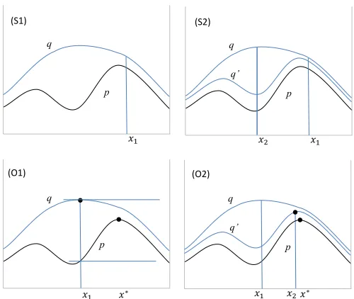
x, otherwise we reject it, (4) we repeat the process with a newx. It can then be shown that this procedure produces an exact sample fromp. Furthermore, the average rate at which it produces these samples, theacceptance rate, is equal toP(X)/Q(X)[Robert and Casella, 2004], where for a (measurable) subsetAofX, we defineP(A)≡R_Ap(x)dµ(x)andQ(A)≡R_Aq(x)dµ(x). In Fig. 1, panel (S1), the acceptance rate is equal to the ratio of the area below thepcurve with that below theqcurve.

2.2 Sampling with OS

The way OS∗_{does sampling is illustrated on the top of Fig. 1. In this illustration, we start} sampling with an initial proposal densityq(see (S1)). Our first attempt producesx1, for which the ratiorq(x1) =p(x1)/q(x1)is close to 1; this leads, say, to the acceptance ofx1. Our second attempt producesx2, for which the ratiorq(x2) =p(x2)/q(x2)is much lower than 1, leading, say, to a rejection. Although we have a rejection, we have gained some useful information, namely thatp(x2)is much lower thanq(x2), and we are going to use that “evidence” to define a new proposalq0_{(see (S2)), which has the following properties:}

• p(x)≤q0_{(x)≤q(x)everywhere onX;} •q0_(x

2)<q(x2).

One extreme way of obtaining such aq0_{is to takeq}0_{(x)equal top(x)forx=x}

2and toq(x) forx6=x2, which, when the spaceXis discrete, has the effect of improving the acceptance rate, but only slightly so, by insuring that any timeq0_{happens to selectx}

2, it will accept it.

p q

𝑥1

p q

𝑥1 𝑥2

q’

(S2) (S1)

p q

𝑥1 𝑥∗

p q

𝑥1

q’

𝑥2𝑥∗ (O2)

(O1)

Figure 1: Sampling with OS∗_{(S1, S2), and optimization with OS}∗_{(O1, O2).}

A better generic way to find aq0_{is the following. Suppose that we are provided with a} small finite set of “one-step refinement actions"aj, depending onqandx2, which are able to move fromqto a newq0

j=aj(q,x2)such that for any suchajone hasp(x)≤q0j(x)≤q(x) everywhere onXand alsoq0

j(x2)<q(x2). Then we will select among theseajmoves the one that is such that theL₁norm ofq0

jis minimal among the possiblej’s, or in other words, such that R

Xq0j(x)dµ(x)is minimal inj. The idea is that, by doing so, we will improve the acceptance rate ofq0

j(which depends directly onkq0jk1) as much as possible, while (i) not having to explore a too large space of possible refinements, and (ii) moving to a representation ofq0

jthat is only slightly more complex thanq, rather than to a much more complex representation for aq0_that could result from exploring a larger space of possible refinements forq.2_{The intuition behind} such one-step refinement actionsajwill become clearer when we consider concrete examples below.

2.3 Optimization with OS

The optimization version of OS∗_{is illustrated on the bottom of Fig. 1, where (O1) shows on} the one hand the functionpthat we are trying to maximize from, along with its (unknown) maximump∗_{, indicated by a black circle on thepcurve, and corresponding tox}∗_{inX. It also} shows a “proposal” functionqwhich is such — analogously to the sampling case — that (1) the

2_{In particular, even if we could find a refinementq}0_{that would exactly coincide withp, and therefore would have the} smallest possibleL1norm, we might not want to use such a refinement if this involved an overly complex representation

functionqis abovepon the whole of the spaceXand (2) it is easy to directly find the pointx1 inXat which it reaches its maximumq∗_{, shown as a black circle on theqcurve.}

A simple, but central, observation is the following one. Suppose that the distance between

q(x1)andp(x1)is smaller thanε, then the distance betweenq(x1)andp∗is also smaller than

ε. This can be checked immediately on the figure, and is due to the fact that on the one hand

p∗_{is higher thanp(x}

1), and that on the other hand it is belowq(x∗), anda fortioribelowq(x1). In other words, if the maximum that we have found forqis at a coordinatex1and we observe thatq(x1)−p(x1)< ε, then we can conclude that we have found the maximum ofpup toε. In the case ofx1in the figure, we are still far from the maximum, and so we “reject”x1, and refineqintoq0_{(see (O2)), using exactly the same approach as in the sampling case, but for one} difference: the one-step refinement optionajthat is selected is now chosen on the basis of how much it decreases, not theL1norm ofq, but the max ofq— where, as a reminder, this max can also be notatedkqk∞, using theL∞norm notation.3

Once thisq0_{has been selected, one can then find its maximum atx}

2and then the process can be repeated withq1=q,q2=q0, ... until the difference betweenqk(xk)andp(xk)is smaller than a certain predefined threshold.

2.4 Sampling

L

vs. Optimization

L

While sampling and optimization are usually seen as two completely distinct tasks, they can actually be viewed as two extremities of a continuous range, when considered in the context of

Lpspaces.

If(X,µ)is a measure space, and iff is a real-valued function on this space, one defines theLp normkfkp, for 1≤p<∞as:kfkp≡

€R

X|f|p(x)dµ(x) Š1/p

[Rudin, 1987]. One also defines theL_∞normkfk∞as: kfk∞≡inf{C≥0 :|f(x)| ≤Cfor almost everyx}, where the right term is called theessential supremumof|f|, and can be thought of roughly as the “max” of the function. So, with some abuse of language, we can simply write:kfk∞≡maxx∈X|f|. The space

Lp, for 1≤p≤ ∞, is then defined as being the space of all functionsf for whichkfkp<∞. Under the simple condition thatkfkp<∞for somep<∞, we have: limp→∞kfkp=kfk∞. The standard notion of sampling is relative toL1. However we can introduce the following generalization — where we use the notationLαinstead ofLpin order to avoid confusion with our use ofpfor denoting the target distribution. We will say that we are performingsampling of a non-negative function f relative to Lα(X,µ), for 1≤α <∞, iff ∈Lα(X,µ)and if we sample — in the standard sense — according to the normalized density distribution ¯f(x)≡ f(x)α

R

Xf(x)αdµ(x) . In the caseα=∞, we will say that we are sampling relative toL_∞(X,µ), iff ∈L_∞(X,µ)and if we are performing optimization relative tof, more precisely, if for anyε >0, we are able to find anxsuch that|kfk∞−f(x)|< ε.

Informally, sampling relative toLα“tends” to sampling withL∞(i.e. optimization), forα tending to∞, in the sense that for a largeα, anxsampled relative toLα“tends” to be close to a maximum forf. We will not attempt to give a precise formal meaning to that observation here, but just note the connection with the idea ofsimulated annealing[Kirkpatrick et al.,

3_{A formal definition of that norm is thatkqk∞is equal to the “essential supremum” ofqover(X,µ)(see below), but}

1983], which we can view as a mix between the MCMC Metropolis-Hastings sampling technique

[Robert and Casella, 2004]and the idea of sampling inLαspaces with larger and largerα’s. In summary, we thus can view optimization as an extreme form of sampling. In the sequel we will often use this generalized sense of sampling in our algorithms.4

2.5 OS

_{as a unified algorithm}

The general design of OS∗_{can be described as follows:}

• Our goal is to OS-sample fromp, where we take the expression “OS-sample” to refer to a generalized sense that covers both sampling (in the standard sense) and optimization.

• We have at our disposal a familyQof proposal densities over the space(X,µ), such that, for everyq∈ Q, we are able to OS-sample efficiently fromq.

• Given a rejectx1relative to a proposalq, withp(x1)<q(x1), we have at our disposal a (limited) number of possible “one-step” refinement optionsq0_{, withp≤q}0_{≤q, and such} thatq0_(x1)<q(x1).

• We then select one suchq0_{. One possible selection criterion is to prefer theq}0_which has the smallest L₁norm (sampling case) or L_∞norm (optimization). In one sense, this is the most natural criterion, as it means we are directly lowering the norm that controls the efficiency of the OS-sampling. For instance, for sampling, ifq0

1andq02are two candidates refinements withkq0

1k1<kq20k1, then the acceptance rate ofq01is larger than that ofq0

2, simply because thenP(X)/Q01(X)>P(X)/Q02(X). Similarly, in optimization, if kq0

1k∞<kq02k∞, then the gap between maxx(q10(x))andp∗is smaller than that between maxx(q02(x))andp∗, simply because then maxx(q10(x))<maxx(q02(x)). However, using this criterion may require the computation of the norm of each of the possible one-step refinements, which can be costly, and one can prefer simpler criteria, for instance simply selecting theq0_{that minimizesq}0_(x

1).

• We iterate until we settle on a “good”q: either (in sampling) one which is such that the cumulative acceptance rate until this point is above a certain threshold; or (in optimization) one for which the ratiop(x1)/q(x1)is closer to 1 than a certain threshold, withx₁being the maximum forq.

The following algorithm gives a unified view of OS∗_{, valid for both sampling and optimization.} This is a high-level view, with some of the content delegated to the subroutinesOS-Sample,

Accept-or-Reject, Update, Refine, Stop, which are described in the text.

Algorithm 1The OS∗_algorithm 1: while notStop(h) do 2: OS-Samplex∼q

3: r←p(x)/q(x)

4: Accept-or-Reject(x,r)

5: Update(h,x) 6: ifRejected(x)then 7: q←Refine(q,x)

8: returnqalong with acceptedx’s inh

On entry into the algorithm, we assume that we are either in sample mode or in optimization mode, and also that we are starting from a proposalqwhich (1) dominatespand (2) from which we can sample or optimize directly. We use the terminologyOS-Sampleto represent either of these cases, whereOS-Sample x∼qrefers to sampling anxaccording to the proposalqor optimizingxonq(namely finding anxwhich is an argmax ofq, a common operation for many NLP tasks), depending on the case. On line (1),hrefers to the history of the sampling so far, namely to the set of trialsx1,x2, ... that have been done so far, each being marked for acceptance or rejection (in the case of sampling, this is the usual notion, in the case of optimization, all but the last proposal will be marked as rejects). The stopping criterionStop(h)will be to stop: (i)

in sampling mode, if the number of acceptances so far relative to the number of trials is larger than a certain predefined threshold, and in this case will return on line (8), first, the list of acceptedx’s so far, which is already a valid sample fromp, and second, the last refinementq, which can then be used to produce any number of future samples as desired with an acceptance ratio similar to the one observed so far; (ii)in optimization mode, if the last elementxof the history is an accept, and in this case will return on line (8), first the valuex, which in this mode is the only accepted trial in the history, and second, the last refinementq(which can be used for such purposes as providing a “certificate of optimality ofx relative top”, but we do not detail this here).

On line (3), we compute the ratior, and then on line (4) we decide to acceptxor not based on this ratio; in optimization mode, we acceptxif the ratio is close enough to 1, as determined by a threshold5_{; in sampling mode, we acceptxbased on a Bernoulli trial of probabilityr.} On line (5), we update the history by recording the trialxand whether it was accepted or not. Ifx was rejected (line (6)), then on line (7), we perform a refinement ofq, based on the principles that we have explained.

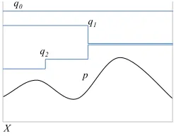
2.6 A connection with A*

A special case of the OS∗_{algorithm, which we call “OS}∗_{with piecewise bounds”, shows a deep} connection with the classical A∗_{optimization algorithm[Hart et al., 1968]and is interesting in} its own right. Let us first focus on sampling, and suppose thatq0represents an initial proposal density, which upper-bounds the target densitypoverX. We start by sampling withq0, and on a first reject somewhere inX, we split the setXinto two disjoint subsetsX1,X2, obtaining a partition ofX. By using the more precise context provided by this partition, we may be able

5_{WhenXis a finite domain, it makes sense to stop on a ratioequalto 1, in which case we have found an exact}

ARSstar1

p q0

X

q1

q2

Figure 2: A connection with A∗_.

to improve our upper boundq0over the whole ofXinto tighter upper bounds on each ofX1 andX2, resulting then in a new upper boundq1over the whole ofX. We then sample usingq1, and experience at some later time another reject, say on a point inX₁; at this point we again partitionX1into two subsetsX11andX12, tighten the bounds on these subsets, and obtain a refined proposalq2overX; we then iterate the process of building this “hierarchical partition” until we reach a certain acceptance-rate threshold.

If we now move our focus to optimization, we see that the refinements that we have just proposed present an analogy to the technique used by A∗_{. This is illustrated in Fig. 2. In A}∗_{, we} start with aconstantoptimistic bound — corresponding to ourq0— for the objective function which is computed at the root of the search tree, which we can assume to be binary. We then expand the two daughters of the root, re-evaluate the optimistic bounds there to new constants, obtaining the piecewise constant proposalq1, and move to the daughter with the highest bound. We continue by expanding at each step the leaf of the partial search tree with the highest optimistic bound (e.g. moving fromq1toq2, etc.).

It is important to note that OS∗_{, when used in optimization mode, is in factstrictly more general}

than A∗_{,for two reasons: (i) it does not assume a piecewise refinement strategy, namely that} the refinements follow a hierarchical partition of the space, where a given refinement is limited to a leaf of the current partition, and (ii) even if such a stategy is followed, it does not assume that the piecewise upper-bounds are constant. Both points will become clearer in the HMM experiments of section 3.1, where including an higher-order n-gram inqhas impact on several regions ofXsimultaneously, possibly overlapping in complex ways with regions touched by previous refinements; in addition, the impact of a single n-gram is non-constant even in the regions it touches, because it depends of the multiplicity of the n-gram, not only on its presence or absence.

3 Some NLP applications of OS

The OS∗_{framework appears to have many applications to NLP problems where we need to} optimize or sample from a complex objective functionp. Let us give a partial list of such situations:

• Efficient decoding and sampling with high-order HMM’s.

– Tagging by joint usage of a PCFG and a HMM tagger; – Hierarchical translation with a complex target language model •Parsing in the presence of non-local features.

•PCFG’s with transversal constraints, probabilistic unification grammars.

We will not explore all of these situations here, but will concentrate on (i) decoding and sampling with high-order HMM’s, for which we provide details and experimental results, and (ii) combining a PCFG with a complex finite-state language model, which we only describe at a high-level. We hope these two illustrations will suffice to give a feeling of the power of the technique.

3.1 High-Order HMMs

Note: An extended and much more detailed version of these HMM experiments is provided in [Carter et al., 2012].

The objective in our HMM experiments is to sample a word sequence with density ¯p(x)

proportional top(x) =plm(x)pobs(o|x), whereplmis the probability of the sequencexunder ann-gram model andpobs(o|x)is the probability of observing the noisy sequence of observations

ogiven that the word sequence isx. Assuming that the observations depend only on the current state, this probability can be written:

p(x) = ` Y

i=1

plm(xi|xii−−1n+1)pobs(oi|xi) . (1)

Approach Taking a tri-gram language model for simplicity, let us definew3(xi|xi−2xi−1) =

plm(xi|xi−2xi−1) pobs(oi|xi). Then consider the observationobe fixed, and write p(x) = Q

iw3(xi|xi−2xi−1). In optimization/decoding, we want to find the argmax ofp(x), and in sampling, to sample fromp(x). Note that the state space associated withpcan be huge, as we

need to represent explicitly all contexts(x_i−2,x_i−1)in the case of a trigram model, and even more contexts for higher-order models.

We definew2(xi|xi−1) =maxxi−2w3(xi|xi−2xi−1), along withw1(xi) =maxxi−1w2(xi|xi−1),

where the maxima are taken over all possible context words in the vocabulary. These quantities, which can be precomputed efficiently, can be seen as optimistic “max-backoffs” of the trigram

xi

i−2, where we have forgotten some part of the context. Our initial proposal is thenq0(x) = Q

iw1(xi). Clearly, for any sequencexof words, we havep(x)≤q0(x). The state space ofq0 is much less costly to represent than that ofp(x).

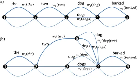
The proposalsqt, which incorporate n-grams of variable orders, can be represented efficiently through weighted FSAs (WFSAs). In Fig. 3(a), we show a WFSA representing the initial proposal

HMMab

two _{𝑤1𝑡𝑤𝑜} dog _{𝑤1𝑑𝑜𝑔}

the 𝑤1𝑡ℎ𝑒 barked

𝑤1𝑏𝑎𝑟𝑘𝑒𝑑

1 2 3 dogs 𝑤1𝑑𝑜𝑔𝑠 4 5

1 5

two

dog

dog

𝑤1𝑡𝑤𝑜

𝑤2𝑑𝑜𝑔|𝑡𝑤𝑜

𝑤1𝑑𝑜𝑔 barked

the

dogs 𝑤1𝑑𝑜𝑔𝑠

dogs

𝑤1𝑑𝑜𝑔𝑠

2 3

6

4

𝑤1𝑡ℎ𝑒

𝑤1𝑏𝑎𝑟𝑘𝑒𝑑

(a)

(b)

Figure 3:An example of an initial q-automaton (a), and its refinement (b).

Consider first sampling, and suppose that the first sample fromq0producesx1=the two dog

barked, marked with bold edges in the drawing. Now, computing the ratiop(x1)/q0(x1)gives a result much smaller than 1, in part because from the viewpoint of the full model p, the trigramthe two dogis very unlikely; i.e. the ratiow3(dog|the two)/w1(dog)is very low. Thus, with high probability,x1is rejected. When this is the case, we produce a refined proposalq1, represented by the WFSA in Fig. 3(b), which takes into account the more realistic bigram weight

w2(dog|two)by adding a node (node 6) for the contexttwo. We then perform a sampling trial withq1, which this time tends to avoid producingdogin the context oftwo; if we experience a reject later on some sequencex2, we refine again, meaning that we identify an n-gram inx2, which, if we extend its context by one (e.g from a unigram to a bigram or from a bigram to a trigram), accounts for some significant part of the gap betweenq1(x2)andp(x2). We stop the refinement process when we start observing acceptance rates above a certain fixed threshold. The case of optimization is similar. Suppose that withq0the maximum isx1=the two dog

barked, then we observe thatp(x1)is lower thanq0(x1), rejectx1and refineq0intoq1. We stop the process at the point where the value ofqt, at its maximumxqt, is equal to the value of patxqt, which implies that we have found the maximum forp.

Setup We evaluate our approach on an SMS-message retrieval task. LetNbe the number of possible words in the vocabulary. A latent variablex∈ {1,· · ·,N}`<sub>represents a sentence</sub> defined as a sequence of`words. Each word is converted into a sequence of numbers based on

a mobile phone numeric keypad, assuming some level of random noise in the conversion. The task is then to recover the original message.

We use the English side of the Europarl corpus[Koehn, 2005]for training and test data (1.3 million sentences). A 5-gram language model is trained using SRILM[Stolcke, 2002]on 90% of the sentences. On the remaining 10%, we randomly select 100 sequences for lengths 1 to 10 to obtain 1000 sequences from which we remove the ones containing numbers, obtaining a test set of size 926.

(d1)

(s1) (s2)

(d2) (s3)

Figure 4: SMS experiments.

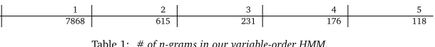
updatingq) that the different n-gram models of size 3, 4 and 5 take to do exact decoding of the sentences of fixed length (10 words) in the test-set. We can see that decoding with larger n-gram models tends to show a linear increase w.r.t.nin the number of iterations taken. Plot (d2) shows the average number of states in the final automatonqfor the same sentences, also showing a linear increase withn(rather than the exponential growth expected if all the possible states were represented). We also display in Table 1 the distribution of n-grams in the final model for one specific sentence of length 10. Note that the total number of n-grams in the full model would be∼3.0×1015_{; exact decoding here is not tractable using existing techniques. By} comparison, our HMM has only 118 five-grams and 9008 n-grams in total.

n: 1 2 3 4 5

q: 7868 615 231 176 118

Table 1: # of n-grams in our variable-order HMM.

Sampling For the sampling experiments, we limit the number of latent tokens to 100. We refine ourqautomaton until we reach a certain fixed cumulative acceptance rate (AR). We also compute a rate based only on the last 100 trials (AR-100), as this tends to better reflect the current acceptance rate. In plot (s3) of Fig. 4, we show a single sampling run using a 5-gram model for an example input, and the cumulative # of accepts (middle curve). It took 500 iterations before the first successful sample fromp.

to highern; for length=10, and forn=3, 4, 5, average number of iterations: 3-658, 4-683, 5-701; averager number of states: 3-1139, 4-1494, 5-1718. In particular the number of states is again much lower than the exponential increase we would expect if using the full underlying state space.

3.2 OS

_{for intersecting PCFG’s with high-order LM’s}

We now move to a high-level description of the application of OS∗_{to an important class of} problems (including hierarchical SMT) which involve the intersection of PCFG’s with high-order language models. The study of similar “agreement-based” problems involving optimization (but not sampling) over a combination of two individual tasks have recently been the focus of a lot of attention in the NLP community, in particular with the application of dual decomposition methods[Rush et al., 2010, Rush and Collins, 2011, Chang and Collins, 2011]. We only sketch the main ideas of our approach.

A standard result of formal language theory is that the intersection of a CFG with a FSA is a CFG

[Bar-Hillel et al., 1961]. This construct can be generalized to the intersection of a Weighted

CFG (WCFG) with a WFSA (see e.g.[Nederhof and Satta, 2003]), resulting in a WCFG. In our case, we will be interested in optimizing and sampling from the intersectionpof a PCFG6_G with a complex WFSAArepresenting a high-order language model. For illustration purposes here, we will suppose thatAis a trigram language model, but the description can be easily transposed to higher-order cases.

Let us denote byxa derivation inG, and byy=y(x)the string of terminal leaves associated withx(the “yield” of the derivationx). The weighted intersectionpofGandAis defined as:

p(x)≡G(x).A(x), whereA(x)is a shorthand forA(y(x)).

Due to the intersection result,pcan in principle be represented by a WCFG, but for a trigram modelA, this grammar can become very large. Our approach will then be the following: we will start by taking the proposalq(0)_{equal toG, and then gradually refine this proposal by}

incorporating more and more accurate approximations to the full automatonA, themselves expressed as weighted automata of small complexity. We will stop refining based on having found a good enough approximation in optimization, or a sampler with sufficient acceptance rate in sampling.

To be precise, let us consider a PCFGG, withP_xG(x) =1, wherexvaries among all the finite derivations relative toG.7_{Let us first note that it is very simple to sample fromG: just expand} derivations top-down using the conditional probabilities of the rules. It is also very easy to find the derivationxof maximum valueG(x)by a standard dynamic programming procedure. We are going to introduce a sequence of proposalsq(0) _{= G,q}(1) _{= q}(0)_.B(1)_{, ...,q}(i+1) ₌ q(i)_.B(i+1)_{, ..., where eachB}(i) _{is a small automaton including some additional knowledge}

about the language model represented byA. Eachq(i)_{will thus be a WCFG (not normalized)}

and refiningq(i)_intoq(i+1)_{will then consist of a “local” update of the grammarq}(i)_{, ensuring a}

desirable incrementality of the refinements.

Analogous to the HMM case, we define: w3(x5|x3x4) =maxx2w4(x5|x2x3x4),w2(x5|x4) =

maxx3w4(x5|x3x4), andw1(x5) =maxx4w4(x5|x4). 6_{A Probabilistic CFG (PCFG) is a special case of a WCFG.}

7_{Such a PCFG is said to be consistent, that is, it is such that the total mass of infinite derivations is null[Wetherell,}

TwoDog1

0 1

two dog

else

else two



1 1

1 1

Figure 5: The “TwoDog” automaton.

Let’s first consider the optimization case, and suppose that, at a certain stage, the grammarq(i)

has already “incorporated” knowledge ofw1(dog). Then suppose that the maximum derivation

x(i)_=argmax(i)_{(x)has the yield:the two dog barked, wherew}

1(dog)is much larger than the more accuratew2(dog|two).

We then decide to updateq(i)_intoq(i+1)_=q(i)_.B(i+1)_{, whereB}(i+1)_{represents the additional}

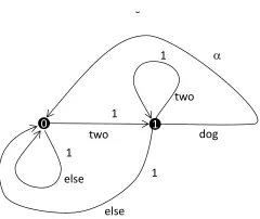
knowledge corresponding tow2(dog|two). More precisely, let us define:

α≡w2_w(dog|two)

1(dog) .

Clearlyα≤1 by the definition ofw1,w2. Now consider the following two-state automaton

B(i+1)_{, which we will call the “TwoDog” automaton:}

In this automaton, the state (0) is both initial and final, and (1) is only final. The state (1) can be interpreted as meaning “I have just produced the wordtwo”. All edges carry a weight of 1, apart from the edge labelleddog, which carries a weight ofα. The “else” label on the arrow from (0) to itself is a shorthand that means: “any word other thantwo”, and the “else” label on the arrow from (1) to (0) has the meaning: “any word other thandogortwo”.

It can be checked that this automaton has the following behavior: it gives a word sequence the weightαk, wherekis the number of times the sequence contains the subsequencetwo dog. Thus, when intersected with the grammarq(i)_{, this automaton produces the grammarq}(i+1)_,

which is such thatq(i+1)_{(x) =q}(i)_{(x)if the yield ofxdoes not contain the subsequencetwo dog,}

but such thatq(i+1)_{(x) =α}k_.q(i)_{(x)if it contains this subsequencektimes. Note that because} q(i)_{had already “recorded” the knowledge aboutw}

1(dog), it now assigns to the worddogin the context oftwothe weightw2(dog|two) =w1(dog).α, while it still assigns to it in all other contexts the weightw1(dog), as desired.8

We will not go here into the detailed mechanics of intersecting the automaton “TwoDog” with the WCFGq(i)_{, (see[Nederhof and Satta, 2008]for one technique), but just note that, because this}

automaton only contains two states and only one edge whose weight is not 1, this intersection can be carried efficiently at each step, and will typically result in very local updates of the grammar.

8_{Note: Our refinements of section 3.1 might also have been seen as intersections between a weighted FSA (rather}

TwoNiceDog1

1 2

two dog

else else

two

0

nice two

else

1 1

1 1

1

1 1



Figure 6: The “TwoNiceDog” automaton.

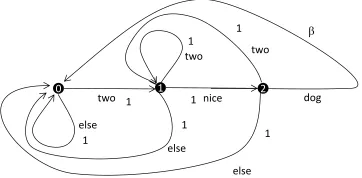
Higher-order n-grams can be registered in the grammar in a similar way. For instance, let’s sup-pose that we have already incorporated in the grammar the knowledge ofw2(dog|nice)and that we now wish to incorporate the knowledge ofw3(dog|two nice), we can now use the following automaton (“TwoNiceDog” automaton), whereβ=w3(dog|two nice)/w2(dog|nice): For optimization, we thus find the maximum x(i) _{of each grammarq}(i)_{, check the ratio} p(x(i)_)/q(i)_(x(i)_{), and stop if this ratio is close enough to 1. Else, we choose an n-gram in} x(i)_{which is not yet registered and would significantly lower the proposalq}(i)_(x(i)_{)if added,}

build the automaton corresponding to this n-gram, and intersect this automaton withq(i)_.

Sampling is done in exactly the same way, the difference being that we now use dynamic programming to compute thesumof weights bottom-up in the grammarsq(i)_{, which is really a}

matter of using the sum-product semiring instead of the max-product semiring.

4 Conclusion

In this paper, we have argued for a unified viewpoint for heuristic optimization and rejection sampling, by using functional upper-bounds for both, and by using rejects as the basis for reducing the gap between the upper-bound and the objective. Bringing together Optimization and Sampling in this way permits to draw inspirations (A∗_{Optimization, Rejection Sampling)} from both domains to produce the joint algorithm OS∗_.

In particular, the optimization mode of OS∗_{, which is directly inspired by rejection sampling,} provides a generic exact optimization technique which appears to be more powerful than A∗_(as argued in section 2.6), and to have many potential applications to NLP distributions based on complex features, of which we detailed only two: high-order HMMs, and an agreement-based model for the combination of a weighted CFG with a language model. As these examples illustrate, often the same dynamic programming techniques can be used for optimization and sampling, the underlying representations being identical, the difference being only a change of semiring.

References

Christophe Andrieu, Nando de Freitas, Arnaud Doucet, and Michael I. Jordan. An introduction to MCMC for machine learning.Machine Learning, 50(1-2):5–43, 2003.

Y. Bar-Hillel, M. Perles, and E. Shamir. On formal properties of simple phrase structure grammars. Zeitschrift für Phonetik, Sprachwissenschaft und Kommunicationsforschung, 14: 143–172, 1961.

Simon Carter, Marc Dymetman, and Guillaume Bouchard. Exact Sampling and Decoding in High-Order Hidden Markov Models. InProceedings of the 2012 Joint Conference on Empirical

Methods in Natural Language Processing and Computational Natural Language Learning, pages

1125–1134, Jeju Island, Korea, July 2012. Association for Computational Linguistics. URL

http://www.aclweb.org/anthology/D12-1103.

Yin-Wen Chang and Michael Collins. Exact decoding of phrase-based translation models through lagrangian relaxation. InEMNLP, pages 26–37, 2011.

M. Dymetman, G. Bouchard, and S. Carter. The OS* Algorithm: a Joint Approach to Exact Optimization and Sampling.ArXiv e-prints, July 2012.

W. R. Gilks and P. Wild. Adaptive rejection sampling for gibbs sampling. Applied Statistics, pages 337–348, 1992.

D. Görür and Y.W. Teh. Concave convex adaptive rejection sampling. Technical report, Gatsby Computational Neuroscience Unit, 2008.

P.E. Hart, N.J. Nilsson, and B. Raphael. A formal basis for the heuristic determination of minimum cost paths. IEEE Transactions On Systems Science And Cybernetics, 4(2): 100–107, 1968. URLhttp://ieeexplore.ieee.org/lpdocs/epic03/wrapper.htm?

arnumber=4082128.

Zhiheng Huang, Yi Chang, Bo Long, Jean-Francois Crespo, Anlei Dong, Sathiya Keerthi, and Su-Lin Wu. Iterative viterbi a* algorithm for k-best sequential decoding. InACL (1), pages 611–619, 2012.

Nobuhiro Kaji, Yasuhiro Fujiwara, Naoki Yoshinaga, and Masaru Kitsuregawa. Efficient Staggered Decoding for Sequence Labeling. InMeeting of the Association for Computational Linguistics, pages 485–494, 2010.

Anthony C. Kam and Gary E. Kopec. Document image decoding by heuristic search. IEEE Transactions on Pattern Analysis and Machine Intelligence, 18:945–950, 1996.

S. Kirkpatrick, C. D. Gelatt, and M. P. Vecchi. Optimization by simulated annealing.Science, 220:671–680, 1983.

Philipp Koehn. Europarl: A parallel corpus for statistical machine translation. InProceedings of

Machine Translation Summit, pages 79–86, 2005.

M.J. Nederhof and G. Satta. Probabilistic parsing as intersection. InProc. 8th International Workshop on Parsing Technologies, 2003.

Slav Petrov.Coarse-to-Fine Natural Language Processing. PhD thesis, University of California at Berkeley, 2009.

K. Popat, D. Bloomberg, and D. Greene. Adding linguistic constraints to document image decoding. InProc. 4th International Workshop on Document Analysis Systems. International Association of Pattern Recognition, December 2000.

Lawrence R. Rabiner. A tutorial on hidden markov models and selected applications in speech recognition.Proceedings of the IEEE, 77(2):257–286, February 1989.

Sebastian Riedel and James Clarke. Incremental integer linear programming for non-projective dependency parsing. InProceedings of the 2006 Conference on Empirical Methods in Natural Lan-guage Processing, pages 129–137, Sydney, Australia, July 2006. Association for Computational Linguistics. URLhttp://www.aclweb.org/anthology/W/W06/W06-1616.

Christian P. Robert and George Casella. Monte Carlo Statistical Methods (Springer Texts in Statistics). Springer-Verlag New York, Inc., Secaucus, NJ, USA, 2004. ISBN 0387212396.

Walter Rudin.Real and Complex Analysis. McGraw-Hill, 1987.

Alexander M. Rush and Michael Collins. Exact decoding of syntactic translation models through lagrangian relaxation. InACL, pages 72–82, 2011.

Alexander M. Rush, David Sontag, Michael Collins, and Tommi Jaakkola. On dual decompo-sition and linear programming relaxations for natural language processing. InProceedings

EMNLP, 2010.

Steven L. Scott. Bayesian methods for hidden markov models: Recursive computing in the 21st century.Journal of the American Statistical Association, 97:337–351, 2002. URLhttp://

EconPapers.repec.org/RePEc:bes:jnlasa:v:97:y:2002:m:march:p:337-351.

Andreas Stolcke. Srilm - an extensible language modeling toolkit. InProceedings of the

International Conference of Spoken Language Processing (INTERSPEECH 2002), pages 257–286,

2002.

Roy W. Tromble and Jason Eisner. A fast finite-state relaxation method for enforcing global con-straints on sequence decoding. InProceedings of the Human Language Technology Conference of the North American Association for Computational Linguistics (HLT-NAACL), pages 423–430, New York, June 2006. URLhttp://cs.jhu.edu/~jason/papers/#tromble-eisner-2006.