Random Process Model for Urban Traffic Flow Using a Wavelet Bayesian Hierarchical Technique

RANDOM PROCESS MODEL FOR TRAFFIC FLOW USING

A WAVELET - BAYESIAN HIERARCHICAL TECHNIQUE

Bidisha Ghosh, Biswajit Basu, and Margaret O’Mahony

Department of Civil, Structural and Environmental Engineering Trinity College, Dublin

Dublin 2

ABSTRACT (148 words)

1 INTRODUCTION

Continuous traffic condition data collection from a large number of junctions in an urban transport network is important for use in the Urban Traffic Control (UTC) systems of today. Although UTC systems are equipped with sophisticated computational and mechanical tools, it is often possible to have several junctions in an urban transport network where traffic conditions (e.g. volume, speed or density) data is not collected regularly (minor intersections). In addition, there can be cases in a network where the data collection system (loop-detector or video imaging system) is not working or is out of service for a considerable period of time. A possible solution to such problems is the development of a traffic volume model which is not directly dependent on recent past and real-time information on traffic flow observations.

This paper develops a random process traffic volume simulation model using wavelet analysis (WA) and Bayesian Hierarchical methodology (BHM). The potential application of the proposed simulation model depends on a novel and unique concept it is not clear to me on the basis of what you have written here that it is unique – can you be more explicit about why it is unique and different to the work of others please of modelling the daily trend underlying the traffic flow over a day in a non-functional manner using discrete WA and subsequently capturing the time-varying variations of the traffic flow observations over the trend implementing a BHM.

(2000), Adeli and Karim (2000), Karim and Adeli (2002), Teng and Qi (2003) and Karim and Adeli (2005)]. It is only recently that researchers in Intelligent Transport Systems (ITS) have shown interest in using this technique for extracting useful information from the existing archived data related to traffic conditions. The traffic flow time-series observations (non-stationary data) are required to be transformed to a stationary process for being modelled using conventional time-series techniques (Chatfield, 2004). The advantage of the application of wavelet analysis is in the inherent capability of accounting for non-stationary time-series. In wavelet analysis based traffic flow modelling, the multi-resolution analysis (MRA) technique (Mallat, 1989) has the potential to be used. This technique, with the advantage of a fast computational algorithm, has been used in feature or pattern extraction at different scales in data/image analysis and can be used as well for multi-scale forecasting of traffic flow. The technique of de-noising using wavelet pre-processing (Sun et al. 2004) has been used by a few researchers for increasing the efficiency of existing short-term traffic flow forecasting models. Chen et al. (2004) combined a wavelet transform with the Markov model to forecast traffic volume. In traffic pattern modelling, varied studies on optimized aggregation level (Qiao et al. 2003); data reduction (Venkatanarayana et al. 2006) and mesoscopic-wavelet model (Ghosh-dastidar and Adeli 2003) have been carried out. Due to very limited research on wavelet based traffic flow modelling in highly congested metropolitan areas there is scope for further exploration in this field.

al., 2002), Bayesian SARIMA models (Ghosh et al. 2007). No literature is available so far on the application of wavelet analysis and subsequent analysis of the randomness using BHM to model traffic flow.

2 TRAFFIC FLOW OBSERVATIONS

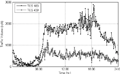
The aim of the study in this paper is to develop a random process traffic volume model to simulate univariate traffic flow time-series data for urban signalised intersections. The proposed model is applied to several intersections in the centre of Dublin to describe and evaluate the methodology. The study at two representative junctions (TCS 183 and TCS 439) is presented in this paper. The univariate traffic flow time-series data used for modelling are obtained from the inductive loop-detectors embedded in the streets of both junctions as part of the urban traffic control (UTC) data collection system used in Dublin. A map of the junctions is given in figure 1. Junction TCS 183 is four-armed with one-way traffic on two approaches. Tara Street (one-way) has four lanes, with traffic flowing from south to north. The traffic volume passing through Tara Street, measured on the loop-detectors numbered 1, 2, 3, 4 are continuously recorded. The junction TCS 439 is a four-armed junction with one-way traffic on both – refers to two – may need to explain why this is not four approaches. The traffic volume passing through Townsend Street, measured on the loop-detectors numbered 1, 2, 3 is used in describing and evaluating the proposed traffic volume model.

from 3 min. to 30 min. are used based on the forecasting algorithms (Xie et al. 2007). In view of the wavelet analysis techniques to be applied on the traffic volume observation a short time interval of 5 min. is chosen for this paper. In the case of an urban transport network, the weekend travel dynamics is inherently different from the travel dynamics during weekdays. In this study, the modeling is essentially carried out on the data observed during weekdays. A plot of the traffic flow data from both junctions in vehicles per hour (vph) against time is shown in figure 2.

3 NON-FUNCTIONAL TREND MODEL

3.1 Multi-Resolution Wavelet Analysis (MRWA)

The wavelet transform provides a time-frequency representation of any signal/time-series data. The basis of wavelet analysis is decomposing a signal into shifted and scaled versions of the original (or mother) wavelet. MRWA uses techniques by which different frequencies of a signal are analyzed with different resolutions by using an efficient numerical algorithm.

The discrete wavelet transform (DWT) (Mallat, 1989) of a signal X(t) consists of the collection of coefficients

 

 

 

 

,

, where, Z=1,2,3... ,

J J k

j j k

c k X t

j k Z

d k X t

            _{ }   (1)

 

₂ 2



₂



j

j j k t t k

 _    _

(2)

which is constructed from the mother-wavelet 

 

t by a time-shift operation (k) and a dilation operation (j). The function _{J k}( )t is a time shifted version of the mother-wavelet scaling function _J( ): t _{J k}( ) = t _J(tk). _J( )t is a low-pass function which can separate the low frequency component of the signal. Thus DWT decomposes a signal into a large timescale (low frequency) approximation and a collection of details at different smaller timescales (higher frequencies).

The original signal can be reconstructed back from the decomposed approximation and the detail components. Thus, the original signal can be represented as,

 

J

 

j

 

j J

X t A t D t



 



(3)

where, AJ

 

t is the reconstruction of the approximation coefficients cJ at level J and

 

j

D t is the reconstruction obtained from the detail coefficients d_j at level j. In the reconstructed approximation (A_J) and in the reconstructed details obtained at each stage/level (D1, D2, D3 … DJ) the numbers of data points remain the same as the

original dataset.

3.2 Trend Model

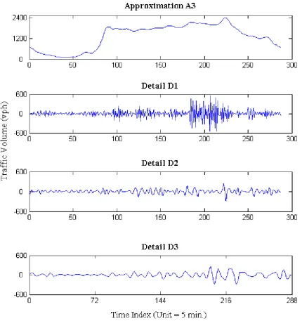
In this study, DWT associated with the basis Daubechies’ 4 (db4) is used to decompose the signal (time-series traffic flow observations) into different time scales. Initially, the original signal is decomposed into approximation coefficients c1 (low

frequency/fluctuations or variability) and detail coefficients d1 (high

frequency/fluctuations or variability). The approximation coefficients c1 (relative low

frequency components) are again decomposed to approximation coefficients c2 (low

fluctuations) and detail coefficients d2 (high fluctuations) at the next level. This

procedure is repeated for further decomposition. The aim of repeating the decomposition procedure is to find an optimum approximation level for extracting the trend in the data. The optimum approximation level is the one in which the reconstructed approximation coefficients, Am (m is the optimum approximation level),

are the optimal smoothed estimate of the traffic flow data which can truly represent the traffic flow pattern on an average day. This is essentially a de-noising technique in signal processing. The local variability in traffic flow observations due to signal control in the urban arterials is considered as the noise (for the mathematical treatment) in this methodology. The traffic flow pattern at any particular approach at any intersection in an urban transport network is similar for weekdays. However, there can be some day-to-day variability due to other factors like, the day of the week, accidents or recurrent congestion in some other part of the transport network etc. These factors are uncontrollable and cannot be modelled as such. So, to obtain a ‘regular trend over an average day’, the Am values over some regular days

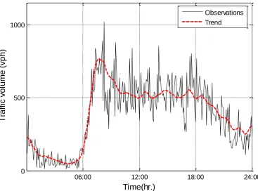
traffic flow time-series observations over 20 days are taken. An average over 20 days of the level 3 reconstructed approximation coefficients for a single day is used to model the representative daily trend for the two chosen approaches from the two chosen intersections. Explain why? The selection of the average coefficients helps to reduce the effect of certain uncontrollable conditions as described before. In figure 4(A) and (B), the ‘regular trend over an average day’ is plotted over the traffic flow observations on 15th June 2005. From the graphs – which graphs? You will need to be specific as to what the reader should be looking at in the figures because it is not clear it can be observed that the simple trend provides a very good approximation of the traffic volume on any arbitrary day.

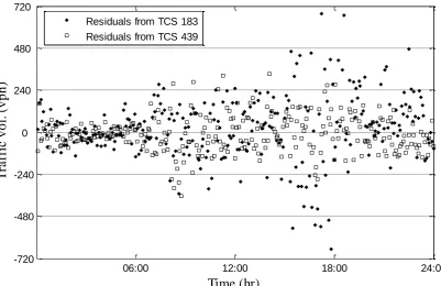
A plot of the residuals from junctions TCS 183 and TCS 439 is given in figure 5. The statistical analyses of the residuals are given in Table 1. Mention in the text some of the more important relevant statistics from this Table. The ‘non-functional daily trend model’ forms the skeleton of a background model for simulating traffic flow at an urban intersection. The modelling of the residual obtained after fitting the trend helps to establish a tight simulation interval.

4 RESIDUAL MODEL

4.1 Crude Residual Model

the residuals is plotted on the histogram in figure 6(A). The normal density fit matches the histogram only crudely. A confidence interval on the ‘regular trend over an average day’ can be provided based on this residual model. The following equation is used in simulating the confidence limit of this background model based on ‘regular trend over an average day’.





where, ~ N 0,

sim  trnd res res res 

y A   (4)

where, y_sim is the simulated traffic volume from the background model; A_trnd is the average value of level three approximation obtained from the trend model; _resis the mean of the residual dataset and _resis the random part of the residuals. _resvalues are randomly generated from a normal distribution with mean zero and standard deviation  which is the sample standard deviation of the residuals. A 95% confidence interval of the residuals is used to form the confidence limit of the background model.

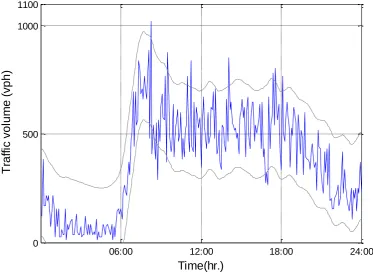
In figure 6(A) and 6(B) the original traffic flow observations on 15th June 2005 are plotted along with simulated confidence intervals from the background model. Most of the observations fall within the confidence limits. This proves that the simplistic background model based on ‘regular trend over an average day’ can be used as an approximate traffic volume simulation model for the intersections where continuous information on traffic conditions is not available.

of the day. The variability is the highest during the evening peak hours. This non-uniform variability signifies that the variance of the residual should not be estimated as a constant parameter for an entire day, but as a variable varying with the time of the day. A bayesian hierarchical model is introduced at this point as a standard statistical method to model the residues with its time varying variance.

4.2 Bayesian Hierarchical Residual Model

In simple words, the basic idea behind the Bayesian hierarchical model is to develop a parametric statistical model with parameters which are represented by other parametric statistical models (i.e. it is doubly stochastic in nature). The essence of hierarchical model is that the dependencies among variables in a statistical model can be defined more easily with a tree-like structure. In the case of a Bayesian hierarchical model, while calculating posterior density (Lee, 199x), priors which themselves depend on other parameters not included in the likelihood function can be accounted for.

In this study, the variance of the residual is dependent on time and has to be modelled accordingly using another parametric statistical model. Hence, the residual obtained from the 5 minute aggregate traffic flow observations on 15-06-2005, after fitting the trend model, are further modelled using a Bayesian hierarchical model to account for the time-varying nature of the variance of the residual dataset. If the R is the vector of the residual, then in a normal hierarchical model,



2



~ N , 1, 2....

t m t t T

R  (5)

{Tx1} where T is the number of time intervals or time instants in a day (for 5 minute aggregate traffic flow observations, T = 288) . The variance2, of the residual dataset R changes with the time of the day. To model this time-varying variability of the variance, the following parametric distribution is proposed.



2



log( )~N log( ), y  (6a)

which leads to ~LN log( ),



y 2



(6b) As  is always positive, a lognormal distribution is taken in equation 6 to ensure that all _t lie within



0,



. The lognormal distribution for each _t is centred at yt with

standard deviation of  . The variances of the high resolution components (sum of level 1, 2 and 3 reconstructed detail coefficients) from the 20 day traffic flow observations calculated over each hour of a day are considered as the initial estimates of the standard deviation of the residual (yt) for that hour of the day. The elements of

the vector y are the same for all time instants within the same hour of the day. The values of the vector y of dimension {Tx1} are calculated from the 20 day dataset and these values are constant for traffic flow observations on an average day at the particular intersection TCS 183 considered in this study. Hence, the Bayesian hierarchical model developed in this study can be considered as applicable to any arbitrary day of the year. The variance 2of the lognormal distribution of vector  is assumed to follow a uniform distribution, within a range

 

0,k





~ U 0, k k

   (7)

subtracting the regular average trend from the traffic flow observations on 15th June 2005.

In the Bayesian hierarchical model, the unknown parameters to be estimated are

( ₁, ₂...₂₈₈) and  . These unknown parameters are represented by a vector



, 1, 2... 288



T

    

ξ . To estimate the vector  the Bayesian estimation technique (Tanner 1996; Lee 1997) is to be used. For the Bayesian inference, the posterior density of the normal hierarchical model is



,



 



,

 

,



p  R t  p  L  R t L   t (8)

where, p



 R t,



is the posterior density of  ; L



 R t,



is the likelihood function of

 and L



 ,t



is the likelihood function of  ; p

 

 is the prior density of

parameter  . According to equation 5, R is assumed to follow a normal distribution. Hence, the likelihood function of given the vector R and the time instant vector t (unit time interval = 5 minute) is





₂ 22

1 1 , exp 2 2 T t t _t t R L          

 R t (9)

Similarly according to equation 6b where is assumed to follow a likelihood function, the likelihood function of given , y and t,







2



2

1 log log 1 , exp 2 2 T t t t _t y

L  

      _           

t (10)

 

p  is equal to a constant as the prior density of is assumed as flat on the range



0,



. Hence, the posterior density from equation 8 is





22



2



2

1 1

log log

1 1

, exp exp

2 2

T T

t t

t

t _{t t} t _t

y R p                        _{ }  

which yields,





2 22



2



2

1

log log

1 1

, exp

2 2

T _{t t}

t T

t _{t t}

y R p        _    _{ } _{ } _  _   _{ }

 R t (11)





2

2

1

2 2 2

1 0 0 0

log log

1 1

... exp ...

2 2 T t t t T T

t _{t t}

y R

d d d

             _   _{   }      _{ }

  _{ } (12)

By integrating out the other unknown parameters except for the one whose distribution is to be estimated, the ‘marginal distributions’ of the each of the unknown parameters can be found out from the integral in equation 12. The computation of the marginal distributions of the unknown parameters in  involves evaluation of a complex integral with problems of high dimensionality. In Bayesian estimation, numerical integrations are often performed to compute the integrations for which the analytical solution is intractable. However, numerical integration may lead to too many approximations and may even become intractable for large models. In many high dimensional cases of Bayesian analysis, certain refinements of Monte Carlo integration methods such as ??? are often used (Carlin1996). There are different non-iterative and non-iterative variations of these refinements. Markov Chain Monte Carlo (MCMC) is the particular iterative variation of Monte Carlo method in which the simulated values are not in iid but are in a Markov chain. In summary, the goal of the MCMC is, given a target distribution (x), a Markov chain {xn} is required to be

In the MCMC method, to simulate the marginal probability distributions for the unknown parameters in the vector



  , ₁, ₂..._T



, given an initial condition



(0) (0) (0) (0)



1 2

, , ... _T

    the following 289 steps are to be iterated (i denotes the

number of iteration):

1. Sample i1from p



i1 ₁( )i , ₂( )i ..._T( )i ,y t_t,



using Gibbs sampler

technique

2. Sample ₁i1using Metropolis Hastings technique

.

.

289. Sample _Ti1using Metropolis Hastings technique

The initial conditions



(0),₁(0),₂(0)..._T(0)



are as follows,

(0)

1

(0) 2

(0) 1

0.5

(log log ) 1

~ Inverse-gamma ,

2 2 T t t t y T          _{ }  _{ }                y (13)

In step 1, the Gibbs sampler technique is used to simulate the distribution of  . From the posterior density in equation 12, a full conditional distribution for  is as follows,









2 1 2 log log 1

, , exp

2 T t t t T y p       _{ }      _{  } _   _{ }  

 R t (14)

0.5 2

T

  (15a)





2

1

0.5 log log T t t t y   





 (15b)

where the density function of the inverse gamma distribution is as follows,

 

_{ }

 1

 

exp p    _   _     

 (15c)

For simplicity the superscript denoting the number of iterations is not used in equations 14 and 15. Steps 2 to 289 are similar in nature and are used to simulate the values of  ₁, ₂..._T in each iteration. The simulation of  is done using Metropolis-Hastings technique. The candidate values of each of the elements of the vector are simulated from the following proposal distribution,

 

2

~ LN log( ),

i  i 

 

 

 y (16)

The simulated value of iat each iteration is accepted following the Metropolis algorithm. According to this algorithm, each simulated value of the elements of the vector iin each iteration is accepted with a probability

 









1 1 1 1 1

1 2 1 1

1 1 1 1 1 1

1 2 1 1

, , ,.... , ,... , ,

, , ,.... , ,... , ,

i i i i i i i

t t t T

t _{i i i i i i i}

t t t T

p p p                              

 R t

R t

(17)

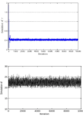
value of about 0.4 and 23 for junction TCS 183 and TCS 439 respectively. Comment on large difference – why so? In the case of the vector of time varying standard deviation , all of the two eighty-eight elements of the vector are simulated separately. Instead of showing a plot of 10000 simulated values of each t, the mean of the simulated values of each t are shown in figure 8(A) and 8(B). The sample standard deviation obtained from the previous Gaussian noise model of the residual is shown as a horizontal line in the same figure. What you are presenting in these figures is not clear – can you be very explicit about what you are trying the reader to interpret from figures 8(a) and 8(b) and explain this in the text. The estimates of obtained from the Bayesian hierarchical model change with the time of the day. The estimates during the peak hours are much more than the estimated values t during the rest of the day and the estimates during the early hours in the morning are the lowest of all. You are presenting very large differences here without sufficient explanation – can you expand on what the differences mean please. The nature of the variability of the variance of the residual conforms to the spread of the residual data points in figure 5 – it is not clear how they conform? .

5 ANALYSES OF RESULTS

In this section a discussion of the 5 minute aggregate traffic flow simulations for junctions TCS 183 and TCS 439 on 15th June 2005 obtained by using the WA-BHM and the WA-Gaussian Noise Models is presented.

In figures 6(A) and 6(B), a 95% confidence interval for traffic flow data from TCS 183 and TCS 439 on 15th _{June 2005 is simulated using the WA-Gaussian Noise}

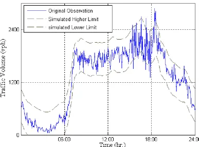
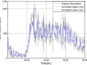
evening and morning peak hours. To illustrate the effectiveness of the WA-BHM model, a 95% confidence interval similar to the Gaussian noise model is constructed on the regular average trend for traffic flow data from intersections TCS 183 and TCS 439 on 15th June 2005. The original 5 minute traffic flow observations on 15th June 2005 are plotted along with the simulated 95% confidence limit in figure 9(A) and 9(B) respectively. Unlike the WA-Gaussian Noise model, all the traffic flow observations on 15-06-2005 – use the same date format throughout the paper fall within the simulated confidence limits. Being a Bayesian method, the confidence limits adapt according to the variability of the residual data. This adaptation proves most effective during the evening peak hours where most of the observations fall outside the simulated limits from the Gaussian noise model. The number of traffic flow observations obtained from TCS 183 and TCS 439 falling outside the simulated interval for both the models are given in Table 2.

minima point errors over a day are seen to be higher than the same during AM peak and PM peak hours. This justifies that the WA-BHM model is more effective in simulating traffic volume during busy peak hours. The justification you have provided is insufficient – can you expand more on why this model is more useful than using the models of others? It would strengthen it if you could compare the results of this model to that of others and give some examples with numbers of why your model is better.

6 CONCLUSIONS

benefits in terms of policy – what difference will using your model make in the real world? – again this relates back to the justification for the research.

.

ACKNOWLEDGEMENT

The research work is funded under the Programme for Research in Third-Level Institutions (PRTLI), administered by the HEA.

In relation to the figures, you will have to present the data so that it can be

clearly interpreted in black and white – some of your figures are relying on

colour to differentiate and this is not acceptable for papers submitted to

REFERENCES

Adeli, H. and A. Samant. (2000) An Adaptive Conjugate Gradient Neural Network-Wavelet Model For Traffic Incident Detection. Computer-Aided Civil Infrastructure Engineering, Vol.15, pp. 251–260.

Adeli, H., and A. Karim. (2000) Fuzzy-Wavelet RBFNN Model for Freeway Incident Detection. Journal of Transportation Engineering, ASCE, Vol. 126, pp. 464–471.

Carlin, B. P. and Louis, T. A. (1996) Bayes and Empirical Bayes Methods for Data Analysis. Chapman & Hall, New York.

Chatfield, C. (2001) Time-Series Forecasting. Chapman and Hall/CRC, London.

Chatfield, C. (2004) The Analysis of Time Series: An Introduction, Sixth Edition. Chapman and Hall/CRC,London.

Chen, S., Wang, W. and Qu, G.(2004) Combining Wavelet Transform and Markov Model to Forecast Traffic Volume, Proceedings of the Third International Conference on Machine Learning and Cybernetics, Shanghai.

Daubechies, I. (1992) Ten Lectures on Wavelets. SIAM, Philadelphia.

Geman, S. and Geman, D. (1984) Stochastic relaxation, Gibbs distributions and Bayesian restoration of images. IEEE Trans. On Pattern Analysis and Machine Intelligence, Vol. 6, pp. 721-741.

Ghosh, B., Basu, B. and O’Mahony, M. M. (2005) Time-Series Modelling for Forecasting Vehicular Traffic Flow in Dublin. 84th Annual Meeting of Transportation Research Board (CD-ROM), TRB, Washington, D. C.

Ghosh, B., Basu, B. and O’Mahony, M. M. (2006a) A Bayesian Time-Series Model For Short-Term Traffic Flow Forecasting. In press, Journal of Transportation Engineering, ASCE.

Ghosh-Dastidar, S. and Adeli, H. (2003) Wavelet-Clustering-Neural Network Model for Freeway Incident Detection. Computer-Aided Civil and Infrastructure Engineering, Vol.18 No.5, pp. 325-338.

Karim, A. and Adeli, H. (2002) Incident Detection Algorithm Using Wavelet Energy Representation of Traffic Patterns. Journal of Transportation Engineering, ASCE, Vol. 128, pp. 232-242.

Mallat, S. (1989) A Theory For Multi-Resolution Signal Decomposition: The Wavelet Representation. IEEE Transactions on Pattern Analysis and Machine Intelligence, Vol. 11(7), pp. 674–693.

Mallat, S. (1998) A Wavelet Tour of Signal Processing (2nd Edition). Academic Press, London.

Mathworks. (2000) Wavelet toolbox for use with MATLAB: User's Guide Version 2. Mathworks Inc. (http://www.mathworks.com)

Metropolis, N., Rosenbluth, A.W., Rosenbluth, M. N., Teller, A. H. and Teller, E. (1953) Equation of State Calculations by Fast Computing Machines. Journal of Chemical Physics, Vol. 21, pp. 1087-1092.

LIST OF FIGURES

1. Diagram of the Junction TCS 183 and TCS 439.

2. Traffic Flow Observations on 15-06-2005 at Junction TCS 183 and TCS 439 3. Reconstructed Approximation Coefficients at Level 3 and Reconstructed

Details Coefficients at Level 1, 2, 3 on 15th June 2005

4. (A) Trend and Original Observations on an Arbitrary Day (15-06-2005) from TCS 183

4. (B) Trend and Original Observations on an Arbitrary Day (15-06-2005) from TCS 439

5. Dot Plot of Residual on 15-06-2005

6. (A) Simulated and Original Traffic Volumes on 15-06-2005 from TCS 439. 6. (B) Simulated and Original Traffic Volumes on 15-06-2005 from TCS 183. 7. Simulations of Values of from TCS 183(upper) and TCS 439 (lower). 8. (A) Simulations of Values of  for TCS 183.

[image:25.595.91.494.74.324.2]

[image:26.595.93.524.86.561.2]

Figure 4(A) Trend and Original Observations on an Arbitrary Day

(15-06-2005) from TCS 183

06:00 12:00 18:00 24:00 0

500 1000

Time(hr.)

T

ra

ff

ic

vo

lu

m

e

(

vp

h

)

Observations Trend

Figure 4(B) Trend and Original Observations on an Arbitrary Day

[image:27.595.92.498.74.367.2] [image:27.595.106.474.443.715.2]

06:00 12:00 18:00 24:00 -720

-480 -240 0 240 480 720

Time (hr)

T

ra

ff

ic

v

o

l.

(

v

p

h

)

[image:28.595.95.497.108.368.2]

Residuals from TCS 183 Residuals from TCS 439

06:00 12:00 18:00 24:00 0

500 1000 1100

Time(hr.)

T

ra

ff

ic

vo

lu

m

e

(

vp

h

)

Figure 6(A) Simulated and Original Traffic Volumes on 15-06-2005 from TCS

439.

You will need to make the lines on these figures distinguishable if published in

black and white as colour will not be an option.

[image:29.595.103.477.90.364.2]

Figure 6(B) Simulated and Original Traffic Volumes on 15-06-2005 from TCS

[image:30.595.100.488.71.357.2]

0 2000 4000 6000 8000 10000 10

15 20 25 30

Iteration

S

im

ul

at

io

n

of

[image:31.595.157.435.70.460.2]

[image:32.595.106.487.86.379.2]

[image:33.595.99.455.124.394.2]

06:00 12:00 18:00 24:00 0

500 1000 1150

Time(hr.)

T

ra

ff

ic

vo

lu

m

e

(

vp

h

)

Original Observation Simulated Higher Limit Simulated Lower Limit

[image:35.595.112.475.102.371.2]

06:00 12:00 18:00 24:00 0

500 1,000

Time (hr.)

T

ra

ff

ic

V

o

lu

m

e

(

v

p

h

)

Maxima Points Minima Points Upper Limit Lower Limit

[image:36.595.104.475.90.376.2]

06:00 12:00 18:00 24:00 0

500 1000

Time (hr.)

T

ra

ff

ic

V

o

lu

m

e

(

v

p

h

)

Maxima Points Minima Points Upper Limit Lower Limit

[image:37.595.100.475.105.358.2]

[image:38.595.95.471.74.357.2]

06:00 12:00 18:00 24:00 0

1,200 2,400

Time (hr.)

T

ra

ff

ic

V

o

lu

m

e

(

v

p

h

)

Maxima Points Minima Points Upper Limit Lower Limit

[image:39.595.104.476.90.364.2]

Mean of Original Observations

(vph)

Standard Deviation of Residuals

(vph)

TCS 183

1301.75 188.28

TCS 439

379.12 103

TCS 183

TCS439

Maxima Points Error

(Over a day)

16.12% 16.9%

Minima Points Error

(Over a day)

19.5% 18.5%

Maxima Points Error

(AM peak 7:30-8:30 am)

8% 8.5%

Minima Points Error

(AM peak 7:30-8:30 am)

11% 11.9%

Maxima Points Error

(PM peak 3:30-4:30 pm)

12.6% 11%

Minima Points Error

(PM peak 3:30-4:30 pm)

15.8% 11%

Points outside

(Trend + BHM model)

0 0

Points outside

(Trend + Gaussian model)

[image:41.595.82.514.82.462.2]

19 16