Abstract—The nominal power of single Wind Energy Conversion Systems (WECS) has been steadily growing, reaching power ratings close to 10MW. In the power conversion stage, medium-voltage power converters are replacing the conventional low-voltage back-to-back topology. Modular Multilevel Converters have appeared as a promising solution for Multi-MW WECSs, due to their modularity, and the capability to reach high nominal voltages. This paper discusses the application of the Modular Multilevel Matrix Converter (M3C) to drive Multi-MW WECSs. The modelling and control systems required for this application are extensively analysed and discussed in this paper. The proposed control strategies enable decoupled operation of the converter, providing maximum power point tracking (MPPT) capability at the generator-side, grid code compliance at the grid-side [including Low Voltage Ride Through Control (LVRT)], and good steady state and dynamic performance for balancing the capacitor voltages in all the clusters. Finally, the effectiveness of the proposed control strategy is validated through simulations and experimental results conducted with a 27 power-cell prototype.
Index Terms—Modular Multilevel Converters, Wind Energy Conversion Systems, Low Voltage Ride Through.
I. INTRODUCTION
IND energy has grown more and at a faster rate than all other renewable energy sources. The wind power
Manuscript received December 16, 2016; revised February 24, 2017; accepted July 03, 2017. This work was supported by FONDECYT under Grant 1140337, AC3E Basal Project grant FB0008 and CONICYT Doctorado Nacional grant 2013-21130721.
M. Diaz and F. Rojas are with the Electrical Engineering Department, University of Santiago of Chile, Santiago 9170124, Chile (e-mail: [email protected]; [email protected]).
R. Cardenas is with the Electrical Engineering Department, University of Chile, Santiago 8370451, Chile (e-mail: [email protected]).
M. Espinoza is with the Electrical Engineering Department, University of Costa Rica, San Jose 11501-2060 UCR, Costa Rica (e-mail: [email protected]).
A. Mora is with the Electrical Engineering Department, Tech. Univ. Fed. Santa Maria, Valparaiso 110-V, Chile (e-mail: [email protected]).
[image:1.612.316.566.235.347.2]J. C. Clare and P. Wheeler are with the Department of Electrical and Electronic Engineering, University of Nottingham, Nottingham NG7 2RD, U.K. (e-mail: [email protected]; [email protected] ).
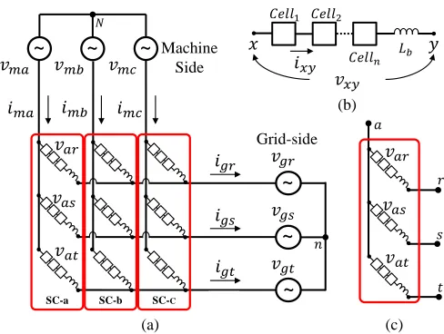
Fig. 1: Proposed topology to drive Multi-MW Wind Turbines
production capacity for the whole world increased from 17.4 GW in 2000 to 432.4 GW in 2015, positioning wind power as a significant and crucial energy source in areas such as Europe, China and the USA [1]. A continual increase in wind power capacity is expected in the immediate future. The European Wind Energy Association (EWEA) has stated that “wind power would be capable of contributing up to 20% of EU electricity by 2020, 30% by 2030 and 50% by 2050” [2].
A significant part of the required future wind power capacity will be installed offshore, due to the presence of higher wind energy and lower environmental impacts. For offshore applications, upscaling wind turbine dimensions, wind park capacities, and electrical infrastructure have become the focus of recent research. A high power wind turbine can reduce the cost structure of offshore WECS [2]. For this reason, wind turbine nominal powers and rotor diameters have increased to 8MW-140m in 2015. In addition, two 10MW WECSs, the Seatitan from WindTec and the Sway 10MW, are expected to be introduced to the market shortly [3], [4].
When the penetration of Wind Energy is high, sudden disconnections of large wind power plants may have a significant influence on the stability of power systems. Therefore, stringent grid codes have been enforced recently, which encompass active power control to support the grid frequency, reactive power control to support the grid voltage, power quality, power controllability, and Fault Ride Through (FRT) capability. FRT requirements regulate the behavior under Low-Voltage Ride-Through, and High-Voltage Ride Through (HVRT) grid voltage conditions and probably represent the primary concern for wind turbine and power converter manufacturers since grid voltage sag-swell are the most common disturbances present in electrical power systems [5]. Despite the trend for Multi-MW Wind Turbines, most of
Blades & Rotor
Modular Multilevel Matrix
Converter
G
Electrical Network PMSG
GEARBOX (OPTIONAL) I
Control of Wind Energy Conversion Systems
Based on the Modular Multilevel Matrix
Converter
Matias Diaz,
Student Member, IEEE,
Roberto Cardenas,
Senior Member, IEEE
,
Mauricio
Espinoza,
Student Member, IEEE,
Felix Rojas, Andres Mora,
Member, IEEE,
Jon C. Clare
,
Senior Member, IEEE,
and
Pat Wheeler
, Senior Member, IEEE
the installed WECSs are based on low-voltage power converters, usually equipped with 1700V IGBT devices for connection to 690V. Therefore, high currents are required at the output of Multi-MW WECS. Thus, medium voltage converter with flexible control strategies could be better suited for this task [3], [6].
In this context, this paper presents a novel application of the M3C to control a high-power WECS, as shown in Fig. 1. The
M3C is a modular AC-AC converter able to reach high-voltage
levels, by the series connection of full-bridge modules. This converter has some advantages compared to conventional two-level topologies for high-power applications, for instance, full modularity, simplicity to reach high voltage levels, control flexibility, power quality and redundancy [7]. In offshore applications, reliability is one of the key parameters. Therefore, the possible redundancy of the M3C, achieved by
adding redundant modules [8], is a major advantage of this topology. The application of M3Cs topologies to WECSs
could lead to reductions in the size of the transformer or even transformerless operation, with the consequent power density increment and weight reduction [9]. In [8], the M3C is
advantageously compared with others high power converter topologies for wind energy applications.
A topology similar to that shown in Fig. 1 was proposed for WECSs in [10], [11]. However, in these papers, the use of cluster inductors is not considered. Therefore, it is assumed that the only five clusters can switch simultaneously to avoid short circuiting the grid-side/machine-side voltage sources (see [10]). Additionally, a Space Vector Modulation (SVM) algorithm is proposed in [10], [11] to synthesise the cluster voltages. Nevertheless, in an M3C composed of n cells there
are 39𝑛 possible switching states, therefore the modulation algorithm discussed in [10], [11], is not feasible when more than two cells per cluster are considered. Furthermore, neither variable speed operation nor grid-connected operation of the M3C are considered in the aforementioned papers.
The contributions of this paper can be summarised as follows:
To the best of our knowledge, this is the first paper where LVRT control systems for M3C applications (see Fig. 1) are
discussed, and experimental results presented.
A decoupled input/output control for an M3C based WECS
is proposed and thoroughly analysed in this paper. Similar to the operation of Back-to-Back converters for WECS applications [4], where the presence of a DC-link allows decoupled control of the AC-DC-AC conversion stages, the proposed control strategy enables the decoupled operation of the grid-side and generator-side control systems.
The regulation of the capacitor voltages is realised using nested control loops, with the outer loops regulating the capacitor voltages (using PI controllers) and the inner control loops regulating the circulating currents. Therefore, the outer control loops regulate the dc-component of the capacitor voltage imbalances with zero steady-state error.
Finally, experimental validation of the proposed control schemes is provided, including variable speed operation, grid code compliance, and capacitor voltage regulation.
The rest of this paper is organised as follows. In Section II, the M3C is discussed. The proposed control systems are
Fig. 2: Modular Multilevel Matrix Converter Topology. (a) Whole converter. (b) M3C Cluster composition. (c) M3C Sub-Converter.
presented in Section III. Then, simulation and experimental results are analysed and extensively discussed in Section IV and Section V, respectively. Finally, an appraisal of the proposed control methodology is presented at the Conclusions.
II. MODULAR MULTILEVEL MATRIX CONVERTER
Fig. 2(a) shows the converter topology used in this work. The M3C has nine clusters connecting the phases of the input
or generator [𝑎, 𝑏, 𝑐 in Fig. 2(a)], to the three phases of the output or grid [𝑟, 𝑠, 𝑡 in Fig. 2(a)]. Each of the nine clusters shown in Fig. 2(a) is composed of 𝑛 Full H-Bridge cells and one inductor (see Fig. 2(b)). As shown in Fig. 2(c), each phase of the generator is connected to the phases (𝑟, 𝑠, 𝑡) using a Sub-Converter (SC).
The switching frequency and voltage levels of a cluster depend on the modulation technique and the number of series-connected cells, leading to a low harmonic distortion when a high number of cells are considered. It is important to note that for this topology, the capacitor voltages of each cell are floating and, therefore, they could charge-discharge during the operation of the converter, particularly when variable speed operation of the generator is considered. Therefore, the capacitor voltages have to be controlled to achieve low voltage ripple around a steady state operating point.
Recently, a decoupled modelling approach for the M3C has
been reported in [12], [13]. In these papers, the basic approach is to use a two-stage-𝛼𝛽0 transformation which is briefly discussed below. Applying Kirchhoff's circuit laws to Fig. 2(a), and assuming that the grid and the generator are ideal voltage sources, the expression of (1) is obtained.
[
𝑣𝑚𝑎 𝑣𝑚𝑏 𝑣𝑚𝑐 𝑣𝑚𝑎 𝑣𝑚𝑏 𝑣𝑚𝑐 𝑣𝑚𝑎 𝑣𝑚𝑏 𝑣𝑚𝑐
] = 𝐿𝑏𝑑 𝑑𝑡[
𝑖𝑎𝑟 𝑖𝑏𝑟 𝑖𝑐𝑟 𝑖𝑎𝑠 𝑖𝑏𝑠 𝑖𝑐𝑠 𝑖𝑎𝑡 𝑖𝑏𝑡 𝑖𝑐𝑡
] + [
𝑣𝑎𝑟 𝑣𝑏𝑟 𝑣𝑐𝑟 𝑣𝑎𝑠 𝑣𝑏𝑠 𝑣𝑐𝑠 𝑣𝑎𝑡 𝑣𝑏𝑡 𝑣𝑐𝑡
] +
[
𝑣𝑔𝑟 𝑣𝑔𝑟 𝑣𝑔𝑟 𝑣𝑔𝑠 𝑣𝑔𝑠 𝑣𝑔𝑠 𝑣𝑔𝑡 𝑣𝑔𝑡 𝑣𝑔𝑡
] + 𝑣𝑁𝑛[
1 1 1 1 1 1 1 1 1
] (1)
The subscript “g” represents grid-side variables and the subscript “m” represents the machine(generator)-side variables. Notice that in (1) the nine cluster voltages 𝑣𝑎𝑟⋯ 𝑣𝑐𝑡 are synthesised by the converter using the modulation indexes obtained from the control systems 𝑟
𝑣𝑎𝑟
𝑣𝑎𝑠
𝑣𝑎𝑡 𝑠
𝑡 𝑎
𝑛 𝐿𝑏
𝑣
𝑖
𝑛
~
~
~
~
~
~
MachineSide
SC-a SC-b SC-C
𝑣𝑚𝑎 𝑣𝑚𝑏 𝑣𝑚𝑐
𝑣𝑔𝑟
𝑣𝑔𝑠
𝑣𝑔𝑡
𝑖𝑔𝑟
𝑖𝑔𝑠
𝑖𝑔𝑡
𝑖𝑚𝑎 𝑖𝑚𝑏 𝑖𝑚𝑐
𝑣𝑎𝑟
𝑣𝑎𝑠
𝑣𝑎𝑡
Grid-side
(a)
(b)
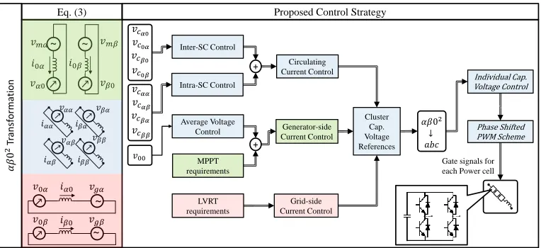
[image:2.612.319.563.51.235.2] [image:2.612.314.561.613.682.2]Fig. 3: Overview of the proposed control strategy.
discussed in this paper. Modulation indexes for each cell are normalised to consider the dc-link voltage variation of each cell capacitor (see Section III.D).
The 𝛼𝛽0 transformation matrix, i.e., 𝛼𝛽0 is defined as:
𝛼𝛽0= √ 3[
1 −1 2⁄ −1 2⁄ 0 √3 2⁄ − √3 2⁄ 1 √2⁄ 1 √2⁄ 1 √2⁄
] (2)
The two-stage-𝛼𝛽0 transformation of the 𝑎𝑏𝑐 signals is realised by the pre-multiplication of (1) by the Cαβ0 matrix and post-multiplication by Cαβ0t . After some manipulations (3) is obtained:
√3 [
0 0 0
0 0 0
𝑣𝑚𝛼 𝑣𝑚𝛽 0 ] = 𝐿𝑏
𝑑 𝑑𝑡[
𝑖𝛼𝛼 𝑖𝛽𝛼 𝑖o𝛼 𝑖𝛼𝛽 𝑖𝛽𝛽 𝑖o𝛽 𝑖𝛼0 𝑖𝛽0 𝑖00
] + [
𝑣𝛼𝛼 𝑣𝛽0 𝑣0𝛼 𝑣𝛼𝛽 𝑣𝛽𝛽 𝑣0𝛽 𝑣𝛼0 𝑣𝛽0 𝑣00] +
√3 [
0 0 𝑣𝑔𝛼 0 0 𝑣𝑔𝛽
0 0 0
] + [
0 0 0
0 0 0
0 0 3𝑣𝑁𝑛
] (3)
where the currents 𝑖𝛼0+ 𝑗𝑖𝛽𝑜 = (𝑖𝑚𝛼+ 𝑗𝑖𝑚𝛽) √3⁄ and the currents 𝑖𝑜𝛼+ 𝑗𝑖𝑜𝛽= (𝑖𝑔𝛼+ 𝑗𝑖𝑔𝛽) √3⁄ . The variables (𝑖𝑚𝛼, 𝑖𝑚𝛽) are dependent on the generator side currents, meanwhile (𝑖g𝛼, 𝑖g𝛽) are dependent on the grid side currents. The currents 𝑖𝛼𝛼, 𝑖𝛽𝛼, 𝑖𝛼𝛽 and 𝑖𝛽𝛽 are not present either at the generator side nor at the grid side and are called “circulating currents”.
III. CONTROL STRATEGY FOR THE M3C BASED WECSS
[image:3.612.309.554.385.459.2]The proposed control strategy provides decoupled regulation of the converter, the input (generator-side), and the output (grid-side). For balanced operation, the average value of each capacitor voltage has to be regulated to an identical reference value. The voltage differences (imbalances) are compensated using circulating currents. As discussed in this section, for the application proposed in this paper four circulating currents are required. These current components are referred to the coordinates of the two-stage-𝛼𝛽0 transformation [see (2-3)] and overview of the proposed control system is presented in Fig. 3, where the following sub-systems are depicted:
Control of the Average Capacitor Voltage
Control of the voltage imbalance in the capacitors
Circulating Current Control.
Generator-side Control System.
Grid-side Control System.
Single Cell Control and Modulation.
The control systems have been designed using the root-locus method and the transfer functions obtained from (3). The circulating current loops have been designed with a bandwidth of about 100Hz and the outer voltage control systems with a bandwidth of 5Hz. A summary of the proposed controllers is shown in Table I with the designed closed-loop bandwidth (Hz) indicated by fn.
TABLE I:SUMMARY OF THE CONTROL SYSTEMS IMPLEMENTED
CONTROL LOOP TYPE 𝑓𝑛[HZ]
Average Voltage 1 PI Controller 10
Cap.Voltage Balancing 4 PI Controllers (outer control loops) 5
Machine-side Current 2 PI Controllers (d-q coordinates) 100
Grid-side current 2 Resonant Controllers 100
Circulating Currents 4 P Controllers (inner control loops) 100
Single-Cell Voltage 27 Proportional Controller 2
The generator is regulated using standard field orientated control techniques, implemented in a synchronous rotating d-q axis. The average value of the cell-capacitor voltages is regulated by imposing an additional component to the generator torque current (i.e. similar to the conventional control methodologies used in back-to-back converters [4]). The grid-side control system regulates the grid-connected operation, power factor regulation and provides FRT compliance.
A. Modelling and Control of the Generator-Side: MPPT
algorithm
The modelling of WECSs and Permanent Magnets Synchronous Generators (PMSGs) have been extensively discussed in the literature [3], [4], [14], [15]. In steady state, the wind turbine operates using an MPPT algorithm, where the generator torque is regulated as:
𝑇𝑒= 𝑘𝑜𝑝𝑡𝜔𝑚→ 𝑃𝑚= 𝑘𝑜𝑝𝑡𝜔𝑚3 (4) where 𝑘𝑜𝑝𝑡is a constant that depends on the blade aerodynamics the gear box ratio and the wind turbine parameters. As presented in [14], the torque-current relationship for a PMSG considering orientation along the rotor flux is:
Intra-SC Control
Cluster Cap. Voltage References Circulating
Current Control
Average Voltage Control
LVRT requirements
~ ~
𝑣𝑚𝛼 𝑣𝑚𝛽
𝑖0𝛼 𝑖0𝛽
𝑣𝛼0 𝑣𝛽0
~
~
𝑣𝑔𝛼
𝑣𝑔𝛽
𝑖𝛼0
𝑖𝛽0
𝑣0𝛼
𝑣0𝛽
𝑣𝛽𝛼
𝑖𝛽𝛼
𝑣𝛼𝛼
𝑖𝛼𝛼
𝑣𝛼𝛽
𝑖𝛼𝛽
𝑣𝛽𝛽
𝑖𝛽𝛽
Tr
an
sf
ormati
on
Proposed Control Strategy
MPPT requirements
+
Eq. (3)
Inter-SC Control
𝑣00
Generator-side Current Control
Grid-side Current Control
+ 𝑣𝑐
𝑣𝑐
𝑣𝑐
𝑣𝑐
𝑣𝑐
𝑣𝑐
𝑣𝑐
𝑣𝑐
Phase Shifted PWM Scheme Individual Cap. Voltage Control
Gate signals for each Power cell 𝛼𝛽0
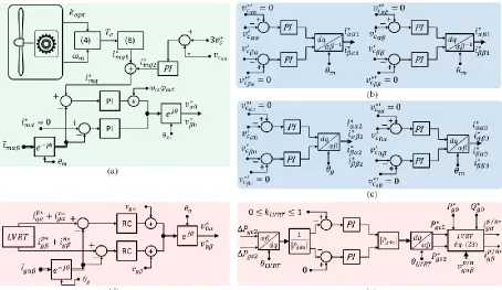
[image:3.612.47.296.394.550.2]Fig. 4: Amplified view of (a) Generator-side control system. (b) Intra-SC capacitor voltage balancing. (c) Inter-SC capacitor voltage balancing. (d) Grid-side control system. (e) LVRT control system.
𝑇𝑒= 3
𝑝 𝜓𝑚𝑟𝑖𝑚𝑞 (5) where p represents the number of pole-pairs in the generator, the PMSG rotor flux is denoted by 𝜓𝑚𝑟 and the generator torque current is 𝑖𝑚𝑞. Replacing (4) in (5), the PMSG current reference for MPPT purposes is calculated as follows:
𝑖𝑚𝑞 ∗ =3 𝑘𝑜𝑝𝑡𝜔𝑚2
𝑝𝜓𝑚𝑟 (6) The proposed control system is presented in Fig. 4(a) where it is shown that the total PMSG torque current is composed of two elements. 𝑖𝑚𝑞 ∗ in (6) and a second component 𝑖𝑚𝑞 ∗ required to regulate one of the voltage components in the M3C. This is discussed later.
B. Control of the M3C
1) Average Capacitor Voltage Control
A single cluster is used to analyse the energy stored in the M3C capacitors [see Fig. 2(b)]. Neglecting internal losses, the
cluster energy 𝑊 is defined as the integral of the cluster power, which is related to the capacitor voltages using:
𝑊 = 𝐶
∑ 𝑣𝑛 𝐶𝑖 (7) Assuming that in each cell the capacitor voltage is operating around a quiescent point 𝑣𝑐𝑖0 ≈ 𝑣𝑐∗, a small signal model of (7) can be derived as:
∆𝑊 = ∑ 𝜕𝑊𝑥𝑦
𝜕𝑣𝑐𝑖 ∆𝑣𝑐𝑖
𝑛 = 𝑣𝑐∗∑ ∆𝑣𝑛 𝑐𝑖= 𝑣𝑐∗∆𝑣𝐶𝑥𝑦 (8) The relationship between the power and the energy of the cluster is obtained from (8) as:
∆𝑃 = 𝑑∆𝑊𝑥𝑦
𝑑𝑡 = 𝑣𝑐 ∗𝑑∆𝑣𝐶𝑥𝑦
𝑑𝑡 (9) Where: 𝑛 is the number of cells in the cluster, ∈ {𝑎, 𝑏, 𝑐}, ∈ {𝑟, 𝑠, 𝑡}, 𝑃 represents the cluster power, 𝑣𝐶𝑥𝑦 is the
addition of all the capacitor voltages in one cluster, 𝑣𝐶∗ is the reference voltage of each cell [assumed as the quiescent point in (8)], represents the capacitance of each capacitor and 𝑊 symbolises the cluster energy.
Using (9), neglecting initial conditions and assuming operation around the aforementioned quiescent point (i.e. 𝑣𝐶𝑥𝑦≈ 𝑛𝑣𝐶∗+ ∆𝑣𝐶
𝑥𝑦), the 9 cluster-capacitor voltages (𝑣𝐶𝑥𝑦)
are obtained as:
[
𝑣𝑐𝑎𝑟𝑣𝑐𝑎𝑠𝑣𝑐𝑎𝑡 𝑣𝑐𝑏𝑟𝑣𝑐𝑏𝑠𝑣𝑐𝑏𝑡
𝑣𝑐𝑐𝑟𝑣𝑐𝑐𝑠 𝑣𝑐𝑐𝑡] = 1 𝐶𝑣𝑐∗∫ [
∆𝑃𝑎𝑟∆𝑃𝑎𝑠 ∆𝑃𝑎𝑡 ∆𝑃𝑏𝑟∆𝑃𝑏𝑠∆𝑃𝑏𝑡 ∆𝑃𝑐𝑟 ∆𝑃𝑐𝑠 ∆𝑃𝑐𝑡 ] 𝑡
0 𝑑𝑡 + 𝑛𝑣𝑐
∗[1 1 11 1 1 1 1 1
] (10)
In 𝑎𝑏𝑐 coordinates, the powers in each cluster are calculated using 𝑃 = 𝑣 𝑖 (see Fig. 2). Applying the two-stage 𝛼𝛽0 transformation to (10) yields:
[
𝑣𝑐 𝑣𝑐 𝑣𝑐0
𝑣𝑐 𝑣𝑐 𝑣𝑐0 𝑣𝑐 0 𝑣𝑐 0 𝑣𝑐00
] = 1 𝐶𝑣𝑐∗∫ [
∆𝑃𝛼𝛼 ∆𝑃𝛽𝛼∆𝑃0𝛼 ∆𝑃𝛼𝛽∆𝑃𝛽𝛽∆𝑃0𝛽 ∆𝑃𝛼0 ∆𝑃𝛽0∆𝑃00 ] 𝑡
0 𝑑𝑡 + [
0 0 0 0 0 0 0 0 3𝑛𝑣𝑐∗] (11) In steady state, when the incremental powers ∆𝑃 ≈ 0 and the capacitor voltages in each cell are equal to 𝑣𝑐∗, the converter is operating in “balanced” conditions. Consequently, most of the voltages (i.e. 𝑣𝑐 , 𝑣𝑐 , 𝑣𝑐 , 𝑣𝑐 , 𝑣𝑐 , 𝑣𝑐 , 𝑣𝑐 , 𝑣𝑐 ) in (11) are equal to zero. The only exception is the
component 𝑣𝑐 = 3𝑛𝑣𝐶
∗. This component is related to the active power flowing into the converter 𝑃00, which can be calculated as the difference between the input and output power, i.e.:
∆𝑃00=3(∆𝑃𝑖𝑛− ∆𝑃𝑜𝑢𝑡) =3( 3
𝑣𝑚𝑞∆𝑖𝑚𝑞− ∆𝑃𝑜𝑢𝑡) ≈
I
current respectively. As shown in (12), the power term ∆𝑃00 is regulated using incremental changes in the generator torque current. The term∆𝑃𝑜𝑢𝑡is considered a disturbance and can be neglected, or used as a feed-forward term, for control purposes. Therefore, for energy balancing purposes, an incremental torque current∆𝑖𝑚𝑞 can be calculated as:
∆𝑖𝑚𝑞 = 2𝐶𝑣𝑐∗
𝑣𝑚𝑞
𝑑∆𝑣𝑐
𝑑𝑡 (13) In this work, the control system regulates the average voltage of all capacitors by using ∆𝑖𝑚𝑞 ∗ , i.e.:
∆𝑖𝑚𝑞 ∗ = −𝐺𝑃𝐼(𝑠)∆𝑣𝑐 = 𝐺𝑃𝐼(𝑠) ( 3𝑛𝑣𝑐
∗− 𝑣
𝑐 ) (14)
where 𝐺𝑃𝐼(𝑠) is the transfer function of a PI controller [see Fig. 4(a)].
2) Control Systems for Balancing the Cap. Voltages
The mean component of the eight voltages in (11) (i.e. 𝑣𝑐 , 𝑣𝑐 , 𝑣𝑐 , 𝑣𝑐 , 𝑣𝑐 , 𝑣𝑐 , 𝑣𝑐 , 𝑣𝑐 ) have to be regulated to
zero in order to balance the converter. The voltage terms 𝑣c ,
𝑣𝑐 , 𝑣𝑐 , 𝑣𝑐 represent capacitor voltage imbalances inside a sub-converter (Intra-SC). The voltage components 𝑣𝑐 ,
𝑣𝑐 , 𝑣𝑐 , 𝑣𝑐 represent imbalances between SCs (Inter-SC).
All these voltage terms could be regulated using either circulating currents or the common mode voltage 𝑣𝑁𝑛 (see [12], [13]). However, the injection of a common-mode voltage could lead to large capacitor-voltage oscillations if a third order harmonic common mode voltage is used, and the generator frequency is one third of the grid frequency (16.3 Hz for a 50 Hz grid) [12]. Therefore, in this work circulating currents alone have been used to regulate the unbalanced voltage components.
The power components in (11) can be expressed as a function of the voltages and currents of the system referred to the two-stage --0 domain (see [12]). Neglecting the voltage drop in the inductance, using 𝑣𝑁𝑛= 0 and denoting “∘” as the Hadamard (element by element) product, the powers in the 𝑎𝑏𝑐-𝑟𝑠𝑡 domain are obtained from (1) as:
[𝑃 ] = ([𝑣𝑚 ] − [𝑣𝑔 ]) ∘ [𝑖 ] (15) Applying the two-stage transformation to (15) and after some manipulations/simplifications (see [12]), the power in the two-stage 0 domain is obtained. For instance, the power component 𝑃𝛼𝛼 can be expressed as:
𝑃𝛼𝛼=3(𝑣𝑚𝛼𝑖𝑔𝛼− 𝑣𝑔𝛼𝑖𝑚𝛼) +√6(𝑣𝑚𝛼𝑖𝛼𝛼− 𝑣𝑚𝛽𝑖𝛽𝛼) −
√6(𝑣𝑔𝛼𝑖𝛼𝛼− 𝑣𝑔𝛽𝑖𝛼𝛽) (16) This component is required to obtain the incremental power ∆𝑃𝛼𝛼, used to regulate 𝑣𝑐 in (11). At this point, some
simplifications to (16) can be considered. If the rotational speed of the WECSs is restricted within a suitable range, then the term (𝑣𝑚𝛼𝑖𝑔𝛼− 𝑣𝑔𝛼𝑖𝑚𝛼) possess components of frequencies 𝜔𝑔± 𝜔𝑚. If the dc-link capacitors are properly designed (see Section III.E) these frequencies do not produce large oscillations in the capacitor voltages.
Therefore, in this work, the circulating currents are designed to generate a non-zero mean active power term in the power 𝑃𝛼𝛼 which can be used to regulate any possible dc-drift or close-to-dc components in this power term. The drift could
be produced, for instance, by non linearities in the converter cells, offsets in the measured signals, etc. Notice that, due to the integral effect produced in the capacitors, even small dc components in the powers of (11) could produce significant voltage imbalances.
Imposing a negative sequence of frequency 𝜔𝑚 (i.e. 𝑖𝛼= 𝑖𝛼𝛼− 𝑗𝑖𝛽α, with 𝑖𝛼𝛼= 𝑖𝑐𝑐𝑐𝑜𝑠𝜃𝑚, 𝑖𝛽𝛼= 𝑖𝑐𝑐𝑠𝑖𝑛𝜃𝑚) in the circulating currents interacting with 𝑃𝛼𝛼, (16) yields to:
𝑃𝛼𝛼= 𝑣𝑚𝑖𝑐𝑐
√6 (cos 𝜃𝑚+ 𝑠𝑖𝑛 𝜃𝑚) ⏞
𝐷𝐶 𝐶𝑜𝑚𝑝𝑜𝑛𝑒𝑛𝑡
− 1
√6 (𝑣𝑔𝛼𝑖𝛼𝛼− 𝑣𝑔𝛽𝑖𝛼𝛽) ⏞ 𝐴𝐶 𝐶𝑜𝑚𝑝𝑜𝑛𝑒𝑛𝑡𝑠 𝜔𝑔±𝜔𝑚
+
3(𝑣𝑚𝛼𝑖𝑔𝛼− 𝑣𝑔𝛼𝑖𝑚𝛼) ⏞ 𝐴𝐶 𝐶𝑜𝑚𝑝𝑜𝑛𝑒𝑛𝑡𝑠 𝜔𝑔±𝜔𝑚
→𝑑∆𝑣𝑐′
𝑑𝑡 =
∆𝑃 ′
𝐶𝑣𝑐∗ ≈ 𝑘 𝑣𝑚𝑖𝑐𝑐 (17) where 𝑘 =
√6𝐶𝑣𝑐∗ and 𝑣𝑐
′
𝛼𝛼is a filtered version of 𝑣𝑐 .
Filtering the AC components in (17) leads to the second expression, which is applied to control the component 𝑣𝑐′
𝛼𝛼. a. Intra-SC balancing current reference calculation:
The same methodology (i.e. neglecting high-frequency components and considering 𝑣𝑁𝑛=0) is used to analyse the dynamic of the incremental voltages ∆𝑣𝑐′𝛼𝛼,∆𝑣𝐶′ , ∆𝑣𝐶′ and ∆𝑣𝐶′ . This yields to:
𝑑 𝑑𝑡 [
∆𝑣𝑐′ 𝛼𝛼 ∆𝑣𝑐′
𝛼𝛽 ∆𝑣𝑐′𝛽𝛼 ∆𝑣𝑐′
𝛽𝛽] = 𝑘1
{[
𝑣𝑚𝛼 0 −𝑣𝑚𝛽 0 0 𝑣𝑚𝛼 0 −𝑣𝑚𝛽 −𝑣𝑚𝛽 0 −𝑣𝑚𝛼 0
0 −𝑣𝑚𝛽 0 −𝑣𝑚𝛼]}[ ∆𝑖𝛼𝛼 ∆𝑖𝛼𝛽 ∆𝑖𝛽𝛼 ∆𝑖𝛽𝛽]
(18)
Therefore, a negative-sequence circulating current component of frequency 𝑚 leads to a non-zero mean active power value, which is manipulated to drive the average component of the unbalanced voltages of (18) to zero. Notice that in (18) circulating currents of frequency 𝑔 could be also applied to the M3C to generate a non-zero mean active power.
However, in this application it is assumed that the WECS has to be synchronised to the grid before being connected. Therefore, before synchronisation well-regulated grid voltages are not available in the cluster voltages and better results can be achieved by using the generator voltages and circulating currents of frequency 𝜔𝑚. As shown in Fig. 4(b), PI controllers regulate the average component of the Intra-SC terms to zero by imposing circulating current references of negative-sequence 𝜔𝑚.
b. Inter-SC balancing current reference calculation
A similar process is carried out to analyse the Inter-SC unbalanced voltages. The dynamics of the unbalanced incremental voltage components are described by:
𝑑 𝑑𝑡 [
∆𝑣𝑐′𝛼0 ∆𝑣𝑐′𝛽0 ∆𝑣𝑐′
0𝛼 ∆𝑣𝑐′0𝛽]
= 1 √3𝐶𝑣𝑐∗[
−𝑣𝑔𝛼 0 𝑣𝑚𝛼
0 −𝑣𝑔𝛽
0 0 𝑣𝑚𝛼
0 −𝑣𝑔𝛼
𝑣𝑚𝛽 0
0 −𝑣𝑔𝛽
0 𝑣𝑚𝛽
]
[ ∆𝑖𝛼𝛼 ∆𝑖𝛼𝛽 ∆𝑖𝛽𝛼 ∆𝑖𝛽𝛽]
(19)
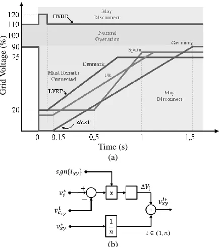
[image:5.612.311.558.636.690.2]Fig. 5: (a) FRT requirements. Voltage profile for faults in Germany, Denmark, UK and Spain. (b) Single cell capacitor voltage control.
In this case, the current references are referred into positive sequence reference frames using the angles 𝜃𝑚 and 𝜃𝑔, as shown in Fig. 4(c).
3) Circulating Current Control
The composite circulating current references are obtained considering the superposition of the Inter-SC and Intra-SC circulating current references. The equation for the circulating current reference 𝑖𝛼𝛼∗ , for example, is:
∆𝑖𝛼𝛼∗ = ∆𝑖
𝛼𝛼1∗ + ∆𝑖𝛼𝛼2∗ + ∆𝑖𝛼𝛼3∗ (20) Similar expressions can be used to obtain the current references ∆𝑖𝛽𝛼∗ , ∆𝑖𝛼𝛽∗ and ∆𝑖𝛽𝛽∗ . In the experimental implementation, the voltage commands required to regulate the four circulating currents are obtained using proportional controllers:
[𝑣𝛼𝛼
∗ 𝑣
𝛽𝛼∗ 𝑣𝛼𝛽∗ 𝑣𝛽𝛽∗
] = −𝑘𝑐𝑐([ 𝑖𝛼𝛼∗ 𝑖
𝛽𝛼∗ 𝑖𝛼𝛽∗ 𝑖𝛽𝛽∗
] − [𝑖𝑖𝛼𝛼 𝑖𝛽𝛼 𝛼𝛽 𝑖𝛽𝛽])
(21)
where 𝑘𝑐𝑐 is the proportional gain required to control the circulating currents with an appropriate dynamic response.
C. Modelling and control of the Grid-Side: LVRT
algorithm
In the last years, stringent grid codes have been enforced for grid-connection of WECS, focusing on power quality, power controllability, and Low Voltage Ride Through (LVRT) capability [16]. As shown in Fig. 5(a), several national grid codes for LVRT demand that WECSs remain connected in the presence of voltage swell-sag, providing grid-voltage support. For the implementation of LVRT control systems, the measured currents and voltages must be separated into positive and negative sequence components to eliminate the power oscillations in the active –or reactive– power injected into the grid. As reported in [17], the power supplied to the grid and the grid voltages/currents are related by (22):
[ 𝑃𝑔0
𝑄𝑔0
𝑃𝑔𝑠2
𝑃𝑔𝑐2]
=
[ 𝑣𝑔𝛼𝑝
𝑣𝑔𝛽𝑝 𝑣𝑔𝛽𝑛
𝑣𝑔𝛼𝑛
𝑣𝑔𝛽𝑝 −𝑣𝑔𝛼𝑝
−𝑣𝑔𝛼𝑛
𝑣𝑔𝛽𝑛
𝑣𝑔𝛼𝑛
𝑣𝑔𝛽𝑛
−𝑣𝑔𝛽𝑝 𝑣𝑔𝛼𝑝
𝑣𝑔𝛽𝑛
−𝑣𝑔𝛼𝑛
𝑣𝑔𝛼𝑝
𝑣𝑔𝛽𝑝 ][ 𝑖𝑔𝛼𝑝
𝑖𝑔𝛽𝑝 𝑖𝑔𝛼𝑛
𝑖𝑔𝛽𝑛]
(22)
Where the superscripts 𝑝, and 𝑛 symbolises the positive and negative-sequence components, respectively. The terms “𝑃𝑔𝑐 ” and “𝑃𝑔𝑠 ” represent double frequency oscillations in active power that can be mitigated using the following references:
[ 𝑖𝑔𝛼𝑝∗ 𝑖𝑔𝛽𝑝∗ 𝑖𝑔𝛼𝑛∗ 𝑖𝑔𝛽𝑛∗ ]
=
[ 𝑣𝑔𝛼𝑝 𝑣𝑔𝛽𝑝 𝑣𝑔𝛽𝑛 𝑣𝑔𝛼𝑛
𝑣𝑔𝛽𝑝 −𝑣𝑔𝛼
𝑝 −𝑣𝑔𝛼𝑛
𝑣𝑔𝛽𝑛 𝑣𝑔𝛼𝑛 𝑣𝑔𝛽𝑛 −𝑣𝑔𝛽𝑝
𝑣𝑔𝛼 𝑝
𝑣𝑔𝛽𝑛 −𝑣𝑔𝛼𝑛
𝑣𝑔𝛼 𝑝 𝑣𝑔𝛽𝑝 ]
−1
[ 𝑃𝑔∗ 𝑄𝑔∗ 𝑃𝑔𝑠2
∗ 𝑃𝑔𝑐2
∗ ]
(23)
If the grid currents calculated from (23), considering 𝑃𝑔𝑐2
∗ = 0, 𝑃 𝑔𝑠2
∗ = 0, are imposed by the control system, the oscillatory active power consumed by the filter inductance is supplied by the M3C. These oscillations are calculated as [17]:
∆𝑃𝑔𝑐2= [2𝑅𝑔′(𝑖𝑔𝛼 𝑝
𝑖𝑔𝛼𝑛 + 𝑖 𝑔𝛽
𝑝
𝑖𝑔𝛽𝑛 ) + 2𝜔𝑔𝐿𝑔′(𝑖𝑔𝛼 𝑝
𝑖𝑔𝛽𝑛 − 𝑖𝑔𝛽 𝑝
𝑖𝑔𝛼𝑛 )] (24) ∆𝑃𝑔𝑠2= [2𝑅𝑔 (𝑖𝑔𝛼
𝑝 𝑖𝑔𝛽𝑛 − 𝑖
𝑔𝛽 𝑝
𝑖𝑔𝛼𝑛 ) + 2𝜔𝑔𝐿𝑔′(−𝑖𝑔𝛼 𝑝
𝑖𝑔𝛼𝑛 − 𝑖𝑔𝛽 𝑝
𝑖𝑔𝛽𝑛 )](25) Where 𝐿𝑔′ and 𝑅𝑔′ are the equivalent inductance and resistance of the grid. The equivalent grid-side inductance is 𝐿´𝑔 = (1 3⁄ )𝐿𝑏+ 𝐿𝑔, where the term (1 3⁄ )𝐿𝑏 corresponds to the parallel connection of the three cluster inductors connected to each of the grid phases, and the term 𝐿𝑔 represents any additional inductance connected between the M3C output and
the grid. As discussed in the previous sections, avoiding voltage oscillations is important in modular multilevel converters where the capacitors are floating. Therefore, to avoid increasing the voltage ripple in the converter, the power oscillations produced in the inductances, i.e. the values of
𝑃𝑔𝑐 ∗ and 𝑃𝑔𝑠 ∗ [see (24)-(25)], have to be supplied by the grid. Then, the values of ∆𝑃gc and ∆𝑃𝑔𝑠 should be considered in the calculation of the reference current in (23), i.e. 𝑃𝑔𝑐2
∗ = −∆𝑃 𝑔𝑐 , 𝑃𝑔𝑠2
∗ = −∆𝑃𝑔𝑠 .
In this section, an enhanced LVRT algorithm, for M3C
applications, is proposed. The control diagram is shown in Fig. 4(d) and Fig. 4(e). The double frequency active power components (∆𝑃𝑔𝑐 and ∆𝑃𝑔𝑠 ) calculated using (24)-(25) are referred to a synchronous frame rotating at twice the grid frequency. Then, PI controllers are used to regulate ∆𝑃𝑔𝑠2 and
∆𝑃𝑔𝑐2 in 𝑑𝑞 coordinates, obtaining the powers 𝑃𝑔𝑠 ∗ and 𝑃𝑔𝑐 ∗ used in (23) [see Fig.4(e)]. To implement (23) the positive and negative components of the currents are estimated using the Delay Signal Cancellation (DSC) method proposed in [18]. Finally, using (23) and the control system shown in Fig. 5, the current references 𝑖𝑔𝛼
𝑝∗
, 𝑖𝑔𝛽𝑝∗, 𝑖𝑔𝛼𝑛∗ and 𝑖𝑔𝛽𝑛∗ are obtained and regulated using Resonant Controllers. The complete control system for the grid converter is presented in Fig. 4(d).
D. Single-Cell Control
The voltage references obtained in the control loops presented above (𝑣𝛼𝛼∗ , 𝑣𝛽𝛼∗ , 𝑣𝛼𝛽∗ , 𝑣𝛽𝛽∗ , 𝑣𝛼0∗ , 𝑣𝛽0∗ , 𝑣0𝛼∗ and 𝑣0𝛽∗ ) are transformed to the natural reference frame using the inverse two-stage 𝛼𝛽0 transform. Then, references 𝑣𝛼𝑟∗ , 𝑣
𝑏𝑟∗ , Time (s)
(a)
(b)
Grid
V
olt
age
(
%
[image:6.612.65.285.52.297.2]I
[image:7.612.332.544.51.399.2]𝑣∗ 𝑣∗ 𝑣∗ 𝑣∗ 𝑣∗ 𝑣∗ 𝑣∗ are obtained for each cluster 𝑐𝑟, 𝑎𝑠, 𝑏𝑠, 𝑐𝑠, 𝑎𝑡, 𝑏𝑡, 𝑐𝑡
[see (1)].
An additional loop (based on a proportional controller) is utilised to regulate the dc-link voltage of each cell within a cluster[19]. The capacitor voltage of each cell𝑖[𝑖∈(1,𝑛)]is compared to the desired value 𝑣𝑐∗. The resulting error is multiplied by the sign of the cluster current (and by the gain kn) producing an incremental voltage ∆𝑉 which is added to the cell reference voltage 𝑣 ∗ /𝑛. The modulation index in each cell is then calculated considering its dc-link voltage value [see Fig. 5(b)]. Finally, phase-shifted PWM is used to synthesise the voltage references. This modulation is simple to implement in a commercial FPGA-based control platform and produces power losses evenly distributed among the cells of the same cluster. Moreover, phase-shifted unipolar modulation generates an output switching frequency of 2n times the carrier frequency [19].
E. Dimensioning of the M3C
To select the correct value of cell capacitance to be utilised in the implementation of the M3C clusters is important [20],
[21]. This capacitance has to be designed to buffer the peak-to-peak energy variations generated by the variable speed operation, maintaining the voltage oscillations inside an appropriate range.
In natural abc, rst frames, the instantaneous power in each cluster is obtained from the Hadamard product of (15) as:
[𝑃 ] = ([𝑣𝑚 ] − [𝑣𝑔 ]) ∘ (1 3⁄ )([𝑖𝑚 ] + [𝑖𝑔 ]) (26) Where ∈ {𝑎, 𝑏, 𝑐} and ∈ {𝑟, 𝑠, 𝑡}. It is assumed that a third of the machine/grid phase currents is circulating in each cluster. Expanding (26), power terms with four oscillating frequencies are obtained: a term of frequency 2𝜔𝑚 ; a term of frequency 2𝜔𝑔; and two power terms of frequencies 𝜔𝑔± 𝜔𝑚 (produced by the input/output cross products, i.e. 𝑣𝑚 𝑖𝑔 − 𝑣𝑔 𝑖𝑚 ). Using (9) the variation in the energy stored in the capacitors could be obtained from these four power terms as:
∆𝑊 = 𝑣𝐶∗∆𝑣𝐶 = ∫ ([𝑃 ]𝜔= 𝜔
𝑚+ [𝑃 ]𝜔= 𝜔𝑔+
𝑡 0 [𝑃 3]𝜔=𝜔
𝑔−𝜔𝑚+ [𝑃 3]𝜔=𝜔𝑔+𝜔𝑚)dt (27)
As discussed in several publications, the capacitor voltage oscillations in the M3C are more difficult to control when the
input/output frequencies have similar values, i.e. 𝜔𝑔− 𝜔𝑚 is relatively small [22]. From (27) the cluster capacitance could be calculated as:
= 𝑘𝑐 ∆𝑊𝑥𝑦
∆𝑣𝑐𝑥𝑦𝑣𝑐∗ (28) where ∆𝑊 is the energy ripple, ∆𝑣𝐶𝑥𝑦 is the maximum
allowable capacitor voltage ripple and 𝑘𝑐 represents an additional safety factor [21]. In this application, kc is selected to slightly oversize the capacitance considering that during LVRT the energy fluctuation in the capacitors could be increased.
In this work, it is assumed that 𝑓𝑔 is 50Hz and the generator is operating between 10-40Hz. Furthermore, the capacitor
Fig. 6: Simulation results during grid faults. (a) Grid Voltages. (b) Grid currents. (c) Generator-side currents. (d) Cluster capacitor voltages.
voltage could be regulated between 100V-155V with a ∆𝑣𝐶𝑥𝑦
of about 15V peak (10% of 155V).
The value of the cluster inductance is relatively simple to calculate by imposing a limit in the ripple of the current (usually set to 10%-15% of the nominal value). This value is calculated as [20][23]:
𝐿𝑏= 0.5(𝑣𝑐∗
𝑛+∆𝑣𝑐𝑥𝑦)
∆𝑖𝑥𝑦𝑓𝑠𝑤 (29)
where ∆𝑖 is the maximum allowable cluster current ripple and 𝑓𝑠𝑤 is the output switching frequency.
IV. SIMULATION RESULTS
A simulation model considering a M3C composed of five
cells per cluster has been implemented using the software PLECS. The design of the high-power converter is depicted in Table II. The parameters of the experimental system are also shown in that Table. It is assumed that a PMSG is connected to the converter input and that medium voltage IGBT devices are used in the M3C implementation (see [24],
I
TABLE II:SIMULATION &EXPERIMENTAL SETUP PARAMETERS
Parameters Simulation Experimental setup
Nominal Power 10 MVA 6kVA
Cells per branch 5 3
Input Voltage/Freq. 5.4kV/10-40Hz 200V/10-40Hz Branch Inductor 1.3 mH 2.5 mH
Single cell C. 8 mF 4.7 mF
Capacitor Voltage 2.4 kV 100-155V Output Voltage/Freq. 5.4kV/50 Hz 185V/50 Hz
Switching frequency 0.7kHz 2.5kHz
When the fault is applied, the active power supplied to the grid is reduced to fulfill the LVRT requirements. As stated in (23), the LVRT control algorithm regulates unbalanced grid- currents to mitigate active power oscillations and to provide reactive power injection, [see Fig. 6(b)]. As a consequence of the fault, the power produced by the generator is reduced as well as the active power fed to the grid [see Fig. 6(c)]. Due to the temporary mismatch between the mechanical input power and the electrical output power, the generator speed could be increased. However, for Multi-MW WECS, the high inertia of the generator; the relatively short duration of the fault (in the milliseconds range); the use of pitch control in the WECS; and the feasibility of using a dc- voltage limiter in each cell reduce the possibility of having large voltage fluctuations in the capacitor voltages during LVRT conditions [see Fig. 6(d)]. Therefore, the control systems for generator-side and grid-side are decoupled during grid-voltage sags, and the dynamic at the machine-side of the M3C remain relatively unaffected [14].
V. EXPERIMENTAL RESULTS
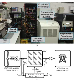
Experimental results for the proposed control methodology have been obtained using a 27-power cell laboratory prototype composed of nine clusters, each comprising the series connection of 3 full-H-bridge modules and one inductor. A photograph of the system is presented in Fig. 7(a) and a diagram is illustrated in Fig. 7(b). Parameters of the experimental system are given in Table II. Because of hardware availability reasons, 2.5mH inductors are used in each cluster, bounding the ripple to about 13% of the maximum cluster current. The system is controlled using a Digital Signal Processor Texas Instrument TMS320C6713 board and 3 Actel ProAsic3 FPGA boards, equipped with 50 14-bit analogue-digital (A/D) channels. A unipolar phase-shifted PWM algorithm generates the 108 switching signals timed via an FPGA. Optical fibre connections transmit the switching signals to the gate drivers of the MOSFET switches. Two programmable AMETEK power supplies emulate the electrical grid and the PMSG. The wind turbine dynamics are programmed in the generator-side power supply (model CSW5550) to emulate a generator operating at variable speed, variable voltage. The grid-side of the M3C is connected to
another power source (Model MX45), which can generate programmable grid sag-swell conditions. The classification of voltage sags presented in [26] (e.g. dip type A, B, etc.) is used in this work. The H-bridges used in the M3C, have been
[image:8.612.314.564.47.316.2]implemented using MOSFET devices of 60A, 300V each one. However, considering the nominal current of the generator- side CSW5550 power supply, the M3C maximum input
Fig. 7: Implemented System (a) Photograph. (b) Diagram.
current has been limited to about 18A peak. Finally, the open loop pre-charge method presented in [27] is used to pre-charge the 27 cell capacitors.
A. Fixed Speed operation
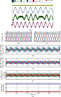
Steady state operation of the experimental prototype for fixed generator frequency is presented in Fig 8. Oscilloscope waveforms of the capacitor voltage 𝑣𝑐𝑎𝑟 , the input voltage 𝑣𝑚𝑎𝑏, the cluster voltage 𝑣𝑎𝑟 and the grid voltage 𝑣𝑔𝑟𝑡 are presented from top to bottom in Fig. 8(a). The generator-side frequency is set to 40 Hz, whereas, the grid frequency is 50 Hz. The cluster voltage 𝑣𝑎𝑟 modulates both (generator and grid) voltages and the different levels produced by the phase shifted modulation are observed. Signals measured using the A/D converters available in the control platform are also presented in Fig. 8(b)-(g). The input and output currents are controlled to 18 A (peak value), and are not much affected by the circulating currents produced by the balancing algorithms. As shown in Fig. 8(b) and Fig. 8(c), the input and output currents present low harmonic distortion (𝑇𝐻𝐷 ≈ 2%) and are balanced. The Inter-SC voltage ripple components (𝑣𝑐0𝛼, 𝑣𝑐0𝛽, 𝑣𝑐𝛼0, 𝑣𝑐𝛽0) are presented in Fig. 8(d), whereas the Intra-SCs ripple components (𝑣𝑐𝛼𝛼, 𝑣𝑐𝛼𝛽, 𝑣𝑐𝛼𝛽, 𝑣𝑐𝛽𝛽) are shown in Fig. 8(e). The eight unbalanced voltage components are successfully regulated inside a ±5V band. For this test, the average value of all the capacitor voltages is regulated to 100V [see Fig. 8(f)]. Fig. 8(g) illustrates the unity power factor operation of the system, in this case, injecting 4kW into the grid.
B. Variable Speed Operation
The operation of a PMSG based variable-speed wind turbine is simulated using a wind speed profile. The frequency and voltage profiles obtained in this simulation are discretised and programmed in the input-side power supply (Model CSW-
M3C
G
CSW5550 AMETEK POWERSOURCE
MX45 AMETEK POWERSOURCE Control Platform
DSP+3 FPGAs
𝑣𝑐𝑥𝑦 𝑖
𝑣𝑔
𝑖
𝑣𝑚
10
3
2
3 Gate Signals
(a)
[image:8.612.66.281.65.175.2][image:9.612.317.554.55.293.2]
(a)
Fig. 8: Experimental results for fixed speed operation. (a) Oscilloscope waveforms operating at 150V. (b)-(g). Exp. results for 𝑣𝐶∗= 100V. (b)
Grid currents. (c) Generator-side currents. (d) Inter-SC components. (e) Intra-SC Components. (f) 27-Capacitor voltages. (g) Active and Reactive Power supplied to the grid.
5550), considering a sampling time of 400 µs. Therefore, the power source generates voltages of variable frequency and magnitudes while emulating the behaviour of a PMSG based wind turbine connected to the M3C input. As shown in Fig.
9(a), the wind speed profile generates a variable rotational speed at the converter input, whereas the grid frequency remains constant. The 27 capacitors have well-regulated voltages during the test [see Fig. 9(b)], even when relatively large variations in the frequency and voltage magnitudes are applied to the M3C-input. The generator-side control system
tracks the maximum power point for each wind velocity, achieving MPPT operation through the regulation of the quadrature current [see (6) and Fig. 9(c)]. Lastly, Fig. 9(d) presents the performance of the grid-side control, which is regulated to operate with unity power factor.
C. Performance of the Control System Considering a
Type A Symmetrical Voltage Dip.
In this test, the MX45 power source is programmed to produce a symmetrical Dip type A, with the phase voltages
Fig. 9: Experimental results for variable speed operation. (a) Grid and generator frequencies. (b) 27-Cells capacitor voltages. (c) Tracking of quadrature input current. (d) Active and Reactive Power supplied to the grid.
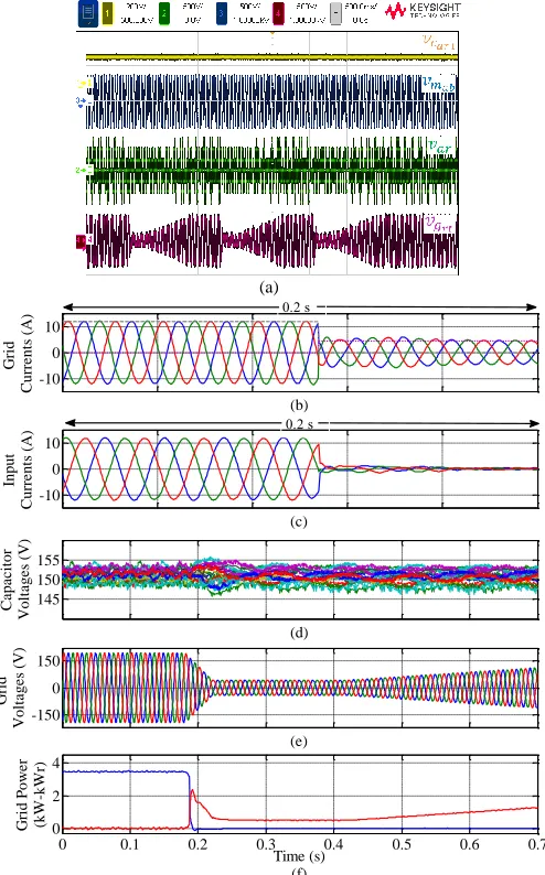
being decreased to a 30% of the nominal value for 0.2s. During the next 0.6s, a profile for the recovery of the grid voltage is applied. Waveforms from the digital scope are shown in Fig. 10(a). The fault is applied three times [an amplified view of the dip is depicted in Fig. 10(e)]. The signals measured by the ADCs of the control platform are presented in Fig. 10(b)-(f). When the fault is applied, the active power reference current is regulated to 0A, and the reactive power current reference is set to 50% of the nominal value. Therefore, the grid current is reduced [see Fig. 10(b)]. The power component of the grid-side current is fed-forward to the generator-side controller. As a consequence of this signal, the generator is no longer controlled using the MPPT algorithm of (6) and the machine side current reference is set to 0A [see Fig. 10(c)]. The performance of the balancing control system to regulate the overall average voltage (𝑣𝑐*=150V) is shown in Fig. 10(d). Good average voltage regulation is observed, and the magnitude of the voltage ripple is less than 4% of the nominal value. As shown in Fig. 10(f), for t 1.9s, the converter supplies only reactive power to the grid.
D. Performance of the Control System Considering a
Type C Asymmetrical Voltage Dip.
The proposed control strategy has been tested considering a Type C Voltage Dip. In this case, two grid phases decrease their voltages to 50% of the nominal value [see Fig. 11(a)]. The output currents are controlled using (24) with 𝑃𝑔∗= 𝑃𝑔𝑐 ∗ = 𝑃𝑔𝑠 ∗ = 0. As discussed in the previous section, the control system regulates the positive and negative currents to mitigate the double-frequency power pulsations. Therefore, the unbalanced grid currents presented in Fig. 11(b) are generated. The 27-cell capacitor voltages are displayed in Fig. 11(c). The voltages are well-regulated using the circulating current discussed in the previous section. Again, -15 0 15 (b) Curre nt (A ) (c) -7 0 7 (d) Int e r-S C U nba l. Ca p. V ol t. (V ) -7 0 7 (e) Int ra -S C U nba l. Ca p. V ol t. (V ) 95 100 105 (f) Ca pa c it or V ol ta ge s (V )
0 0.2 0.4 0.6 0.8 1
0 2 4 Time (s) (g) G ri d P ow e r (kW -kW r) 0.1s 0.1s 20 35 50 (a) M a c hi ne /G ri d F re que nc y (H z ) 0 4 8 12 (c) Q ua dra ture M a c hi ne Cur re nt (A )
0 4 8 12 16 20
[image:9.612.47.297.57.453.2](a)
Fig. 10: Experimental Results. (a) Oscilloscope Waveforms. (b) Grid Currents. (c) Generator-side Currents (d) 27-Capacitor Voltages. (e) Amplified view of grid voltages (f) Active and reactive power injected into the grid.
the magnitude of the voltage ripple is less than 7% of the reference voltage (150V). As shown in Fig. 11(d), when the grid currents are regulated using (24), the active power supplied to the grid is regulated to zero [see Fig. 11(d)] and the converter supplies only reactive power to the grid. However, in this case, the power oscillations required by the filters are provided by the converter, and this could increase the voltage oscillations in the M3C-capacitors during LVRT.
Alternatively, the control system depicted in Fig. 5 can be applied to reduce the power oscillation in the converter. The experimental results are shown in Fig. 11(e). In this case, the active power oscillations in the converter are successfully reduced by a factor of approximately three compared to the oscillations obtained with the conventional LVRT.
VI. CONCLUSIONS
This paper has described the application of a modular multilevel matrix converter for variable speed WECS. Due to the topology characteristics, such as modularity and scalability, this converter is well suited for high power
appli-Fig. 11: Experimental Results. (a) Grid Voltages. (b) Grid Currents. (c) 27-H- Bridge Cells Capacitor Voltages. (d) Active and reactive power injected into the grid using the conventional LVRT (e) Active power oscillations at M3C terminals. Blue line for the conventional LVRT algorithm, and green line for the proposed LVRT algorithm.
cations.Extensive discussion on the modelling and control of the M3C has been presented, introducing a decoupled control
strategy based on a two-stage αβ0 transformation. The proposed control strategy has been validated using a 27-Cell M3C prototype of 4kW. The energy balancing control, the
LVRT strategy and then control of the circulating current have all presented excellent dynamic performance, even when very demanding symmetrical and asymmetrical faults have been experimentally applied to the prototype.
REFERENCES
[1] Global Wind Energy Council, “Global Wind Statistics 2015.” [2] The European Wind Energy Association, “UpWind: Design limits and
solutions for very large wind turbines,” 2016.
[3] V. Yaramasu, B. Wu, P. C. Sen, S. Kouro, and M. Narimani, “High-power wind energy conversion systems: State-of-the-art and emerging technologies,” Proc. IEEE, vol. 103, no. 5, pp. 740–788, 2015. [4] M. Liserre, R. Cardenas, M. Molinas, J. Rodriguez, R. Cárdenas, M.
Molinas, J. Rodríguez, R. Cardenas, M. Molinas, and J. Rodriguez, “Overview of Multi-MW Wind Turbines and Wind Parks,” IEEE Trans. Ind. Electron., vol. 58, no. 4, pp. 1081–1095, Apr. 2011. [5] O. S. Senturk and A. M. Hava, “A simple sag generator using SSRs,”
IEEE Trans. Ind. Appl., vol. 48, no. 1, pp. 172–180, Sep. 2012. [6] H. Abu-Rub, J. Holtz, and J. Rodriguez, “Medium-Voltage Multilevel
Converters—State of the Art, Challenges, and Requirements in Industrial Applications,” IEEE Trans. Ind. Electron., vol. 57, no. 8, pp. 2581–2596, Aug. 2010.
[7] A. J. Korn, M. Winkelnkemper, P. Steimer, and J. W. Kolar, “Direct modular multi-level converter for gearless low-speed drives,” in Power Electronics and Applications (EPE 2011), Proceedings of the 2011-14th European Conference on, 2011, no. direct MMC, pp. 1–7. [8] J. Kucka, D. Karwatzki, and A. Mertens, “Optimised operating range of
modular multilevel converters for AC/AC conversion with failed modules,” in 2015 17th European Conference on Power Electronics and Applications, EPE-ECCE Europe 2015, 2015, pp. 1–10.
[9] T. M. Iversen, S. S. Gjerde, and T. Undeland, “Multilevel converters for a 10 MW, 100 kV transformer-less offshore wind generator -10
0 10
(b)
G
ri
d
Curre
nt
s (A
)
-10 0 10
(c)
Input
Curre
nt
s (A
)
145 150 155
(d)
Ca
pa
c
it
or
V
ol
ta
ge
s (V
)
-150 0 150
(e)
G
ri
d
V
ol
ta
ge
s (V
)
0 0.1 0.2 0.3 0.4 0.5 0.6 0.7
0 2 4
Time (s) (f)
G
ri
d P
ow
e
r
(kW
-kW
r)
0.2 s
0.2 s
-20 0 20
(b)
G
ri
d
Curre
nt
s (A
)
-200 0 200
(a)
G
ri
d
V
ol
ta
ge
s (V
)
140 150 160
(c)
Ca
pa
c
it
or
V
ol
ta
ge
s (V
)
0 0.1 0.2 0.3 0.4 0.5 0.6 0.7
0 2 4
Time (s) (d)
G
ri
d P
ow
e
r
(kW
-kV
A
r)
0.1 0.15 0.2 0.25 0.3
-0.2 0 0.2
(e)
M
3C A
c
t. P
ow
e
r
O
sc
il
la
t. (kW
)
PM3C kLVRT=1 PM3C kLVRT=0
P
[image:10.612.51.298.54.451.2]system,” in 2013 15th European Conference on Power Electronics and Applications, EPE 2013, 2013, pp. 1–10.
[10] R. Erickson, S. Angkititrakul, and K. Almazeedi, “A New Family of Multilevel Matrix Converters for Wind Power Applications: Final Report,” 2006.
[11] R. W. Erickson and O. A. Al-Naseem, “A new family of matrix converters,” in IECON’01. 27th Annual Conference of the IEEE Industrial Electronics Society (Cat. No.37243), 2001, vol. 2, pp. 1515– 1520.
[12] W. Kawamura, M. Hagiwara, and H. Akagi, “Control and Experiment of a Modular Multilevel Cascade Converter Based on Triple-Star Bridge Cells,” IEEE Trans. Ind. Appl., vol. 50, no. 5, pp. 3536–3548, Sep. 2014.
[13] F. Kammerer, J. Kolb, and M. Braun, “Fully decoupled current control and energy balancing of the Modular Multilevel Matrix Converter,” in
15th International Power Electronics and Motion Control Conference and Exposition, EPE-PEMC 2012 ECCE Europe, 2012, p. LS2a.3-1-LS2a.3-8.
[14] M. Chinchilla, S. Arnaltes, and J. C. Burgos, “Control of permanent-magnet generators applied to variable-speed wind-energy systems connected to the grid,” IEEE Trans. Energy Convers., vol. 21, no. 1, pp. 130–135, Mar. 2006.
[15] M. Espinoza, R. Cardenas, M. Diaz, and J. Clare, “An Enhanced dq-Based Vector Control System for Modular Multilevel Converters Feeding Variable Speed Drives,” IEEE Trans. Ind. Electron., no. November, pp. 1–1, 2016.
[16] F. Iov, A. D. Hansen, P. Sørensen, and N. A. Cutululis, “Mapping of grid faults and grid codes,” Wind Energy, vol. 1617, no. July, pp. 1–41, 2007.
[17] M. Diaz, R. Cardenas, P. Wheeler, J. Clare, and F. Rojas, “Resonant Control System for Low-Voltage Ride-Through in Wind Energy Conversion Systems,” IET Power Electron., vol. 9, no. 6, pp. 1–16, May 2016.
[18] R. Cardenas, M. Diaz, F. Rojas, and J. Clare, “Fast Convergence Delayed Signal Cancellation Method for Sequence Component Separation,” IEEE Trans. Power Deliv., vol. 30, no. 4, pp. 2055–2057, Aug. 2015.
[19] H. Akagi, S. Inoue, and T. Yoshii, “Control and Performance of a Transformerless Cascade PWM STATCOM With Star Configuration,”
IEEE Trans. Ind. Appl., vol. 43, no. 4, pp. 1041–1049, 2007.
[20] J. Kolb, F. Kammerer, and M. Braun, “Dimensioning and design of a modular multilevel converter for drive applications,” in 15th International Power Electronics and Motion Control Conference and Exposition, EPE-PEMC 2012 ECCE Europe, 2012, p. LS1a-1.1-1-LS1a-1.1-8.
[21] F. Kammerer, J. Kolb, and M. Braun, “Optimization of the passive components of the Modular Multilevel Matrix Converter for Drive Applications,” in PCIM Europe: Proceedings of the International Exhibition and Conference for Power Electronics, Intelligent Motion, Renewable Energy and Energy Management, Nuremberg, May 8 - 10, 2012, 2012.
[22] Y. Okazaki, W. Kawamura, M. Hagiwara, H. Akagi, T. Ishida, M. Tsukakoshi, and R. Nakamura, “Which is more suitable for MMCC-based medium-voltage motor drives, a DSCC inverter or a TSBC converter?,” in 2015 9th International Conference on Power Electronics and ECCE Asia (ICPE-ECCE Asia), 2015, pp. 1053–1060. [23] B. Li, S. Zhou, D. Xu, R. Yang, D. Xu, C. Buccella, and C. Cecati, “An
Improved Circulating Current Injection Method for Modular Multilevel Converters in Variable-Speed Drives,” IEEE Trans. Ind. Electron., vol. 63, no. 11, pp. 7215–7225, Nov. 2016.
[24] J. G. Bauer, M. Wissen, T. Gutt, J. Biermann, C. Schäffer, G. Schmidt, and F. Pfirsch, “New 4.5 kV IGBT and diode chip set for HVDC Transmission Applications,” in PCIM Europe 2014.
[25] A. Chakraborty, “Advancements in power electronics and drives in interface with growing renewable energy resources,” Renew. Sustain. Energy Rev., vol. 15, no. 4, pp. 1816–1827, May 2011.
[26] M. H. J. Bollen, “Characterisation of voltage sags experienced by three-phase adjustable-speed drives,” IEEE Trans. Power Deliv., vol. 12, no. 4, pp. 1666–1671, 1997.
[27] J. Qin, S. Debnath, and M. Saeedifard, “Precharging strategy for soft startup process of modular multilevel converters based on various SM circuits,” in 2016 IEEE Applied Power Electronics Conference and Exposition (APEC), 2016, pp. 1528–1533.
Matias Diaz (S’15) was born in Santiago, Chile. He received the B.Sc. and M.Sc. degrees in electrical engineering from the University of Santiago, Santiago, Chile, in 2011. He is currently working toward a dual Ph.D. degree at the University of Nottingham, Nottingham, U.K., and at the University of Chile, Santiago, Chile. From 2013 to 2015, he was the Subdirector of the School of Engineering, Duoc-UC, Santiago. He is currently a Lecturer with the University of Santiago. His main research interests include the control of wind energy conversion systems and multilevel converters.
Roberto Cardenas (S’95–M’97–SM’07) was born in Punta Arenas, Chile. He received the B.Sc. degree in electrical engineering from the University of Magallanes, Punta Arenas, in 1988, and the M.Sc. degree in electronic engineering and the Ph.D. degree in electrical and electronic engineering from the University of Nottingham, Nottingham, U.K., in 1992 and 1996, respectively. From 1989 to 1991 and 1996 to 2008, he was a Lecturer with the University of Magallanes. From 1991 to 1996, he was with the Power Electronics Machines and Control Group, University of Nottingham. From 2009 to 2011, he was with the Electrical Engineering Department, University of Santiago. He is currently a Professor of power electronics and drives in the Electrical Engineering Department, University of Chile, Santiago, Chile. His main research interests include control of electrical machines and variable-speed drives.
Mauricio Espinoza (S’15) was born in Alajuela, Costa Rica. He received the B.Sc. and Lic. degrees in electrical engineering from the University of Costa Rica in 2010 and 2012 respectively. From 2010-2014 he was a lecturer at the University of Costa Rica. Actually, he is
pursuing a Ph.D. degree at the University of
Chile, Chile. During his career, he has worked in research projects related to Modular Multilevel Converters, machine modelling and control systems for power electronics.
Andrés Mora (S'14) was born in Santiago, Chile, in 1984. He received the Eng. and M.Sc degrees in electrical engineering from the Universidad Técnica Federico Santa María (UTFSM), Valparaíso, Chile, in 2010. He is currently working toward the Ph.D degree in electrical engineering at the Universidad de Chile, Santiago, Chile. Since 2011, he has been an Assistant Professor with Department of Electrical Engineering, UTFSM. His research interests include power converters and control of electrical machines.
I
Jon C. Clare (M’90–SM’04) was born in Bristol,
U.K., in 1957. He received the B.Sc. and Ph.D. degrees in electrical engineering from the University of Bristol, Bristol. From 1984 to 1990, he was a Research Assistant and Lecturer with the University of Bristol, where he was involved in teaching and research on power electronic systems. Since 1990, he has been with the Power Electronics, Machines and Control Group, University of Nottingham, Nottingham, U.K., where he is currently a Professor of power electronics. His research interests include power-electronic converters and modulation strategies, variable-speed-drive systems, and electromagnetic compatibility.
Prof Pat Wheeler received his BEng [Hons] degree in 1990 from the University of Bristol, UK. He received his PhD degree in Electrical Engineering for his work on Matrix Converters from the University of Bristol, UK in 1994. In 1993 he moved to the University of Nottingham and worked as a research assistant in the Department of Electrical and Electronic Engineering. In 1996 he became a Lecturer in the Power Electronics, Machines and Control Group at the University of Nottingham, UK. Since January 2008 he has been a Full Professor in the same research group. He is currently Head of the Department of Electrical and Electronic Engineering at the University of Nottingham. He is an IEEE PELs ‘Member at Large’ and an IEEE PELs Distinguished Lecturer. He has published 400 academic publications in leading international conferences and journals.

![Fig. 4(a)]. 2) Control Systems for Balancing the Cap. Voltages The mean component of the eight voltages in (11) (i.e.](https://thumb-us.123doks.com/thumbv2/123dok_us/8568622.367800/5.612.311.558.636.690/fig-control-systems-balancing-cap-voltages-component-voltages.webp)