Identification of particle laden flow features from wavelet decomposition

Identification of particle-laden flow features from

wavelet decomposition

A. Jackson∗, B. Turnbull∗∗

Geohazards & Earth Processes Group, Faculty of Engineering, University of Nottingham, NG7 2RD. UK

Abstract

A wavelet decomposition based technique is applied to air pressure data ob-tained from laboratory-scale powder snow avalanches. This technique is shown to be a powerful tool for identifying both repeatable and chaotic features at any frequency within the signal. Additionally, this technique is demonstrated to be a robust method for the removal of noise from the signal as well as being capable of removing other contaminants from the signal. Whilst powder snow avalanches are the focus of the experiments analysed here, the features identified can provide insight to other particle-laden gravity currents and the technique described is applicable to a wide variety of experimental signals.

Keywords: wavelet, particle-laden gravity current, filtering, signal processing

1. Introduction

Particle-laden gravity currents exist in many different forms throughout na-ture, examples include powder snow avalanches, turbidity currents and pyroclas-tic flows. These geophysical phenomena typically exhibit a dense, more granular flow, however here we are concerned with the suspended material, where the in-terplay between particle and interstitial fluid flow is paramount. These currents can be extremely destructive, due to the large changes in pressure over very short time periods, capable of subjecting structures to high stresses. The forces exerted by these pressure changes can be up to four times that exerted through hydrostatic pressure variation within the flows [21]. It is therefore of interest to study fluid pressure signals obtained from particle-laden gravity currents in order to gain a better insight into their internal structure and dynamics.

Here we are primarily motivated by powder snow avalanches (PSAs), but the techniques discussed are equally applicable to other forms of particle-laden

∗_{Current Address}

Health and Safety Laboratory, Harpur Hill, Buxton, Derbyshire, SK17 9JN. UK

∗∗_{Corresponding author}

gravity current.

Due to their dangerous nature and unpredictability, obtaining air pressure data from natural PSAs is extremely difficult. Laboratory-scale physical models are therefore a useful tool for collecting repeatable and controlled data.

1.0.1. Similarity criteria

PSAs are non-Boussinesq, since the particulate material (snow) is relatively dense compared with the ambient fluid (air) and the particles thus carry a significant proportion of the current’s momentum.

Three different particulate materials have been used in order to create particle-laden gravity currents that have density ratios that fall within the non-Boussinesq regime - a sawdust and aluminium mixture [5], Expanded polystyrene (EPS) [18, 20] and powder snow [20].

The particle Reynolds number

Rep=

ρaudp

µ , (1)

is the ratio of the viscous and form drag forces (per unit volume) of a particle

with diameterdp and velocityuin ambient fluid of viscosityµ and densityρa

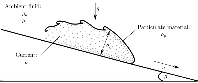
(Figure 1). The particle Reynolds number determines whether the drag is

dom-inated by viscous or pressure forces. PSAs typically have a Rep≈3000 meaning

viscous drag forces play a minor role compared with the form drag of the

par-ticle. For values 500<Rep<105 the drag coefficient for a spherical particle is

essentially independent of Rep [15] and so within this range of Rep drag forces

in PSAs will be well modelled. It should be noted that both the natural and model powder snow particles are henceforth assumed to be spherical. While it is unlikely that the particles are perfectly spherical, a particle’s eccentricity will

only have an effect on it’s drag coefficient when Rep>≈105 [15], which is well

above the typical values of Repobserved in natural PSAs.

Laboratory-scale snow-air and polystyrene-air models have a Rep≈150 due

to the currents reaching much lower speeds than PSAs. Therefore viscous forces between the air and snow/polystyrene particles will have a greater effect on these

flows than in a PSA. However, for these models Rep is still large enough that

form drag will be dominant and viscous drag forces can be considered small,

especially compared with Bozhinskiy and Sukhanov’s experiments (Rep≈0.1),

where the particles are so fine that drag force is dominated by viscous forces. The Richardson number (Ri) is the ratio of potential energy to kinetic energy of particles at the sheared interface between two fluids. The Richardson number

for a layer of heighthc and velocityuon a slope at angleθto the horizontal is

Ri =g

0_h ccosθ

u2 . (2)

The reduced gravity is g0 = g∆ρ/ρa, where ∆ρ = ρ−ρa with ρ and ρa the

densities of the current and the ambient fluid respectively (Figure 1). The

h_c g

u

θ

Particulate material: ρp

Ambient fluid: ρa µ

Current: ρ

Figure 1: Schematic diagram of a particulate gravity current of heighthc, density ρ and

velocityutravelling down a plane inclined at an angleθto the horizontal. Ambient fluid has

densityρaand viscosityµ, and individual particles have densityρp.

Ri value is low, a dense flow will entrain air on the upper surface and become suspended. If the Ri value remains low the current will maintain the particles in suspension and further entrain air. The value of Ri for natural PSAs is typically

≈1, meaning that the powder snow particles become, and remain suspended.

Due to the lower velocities of laboratory-scale snow-air and polystyrene-air flows, very high slope angles have to be used in order to achieve values of Ri identical to those observed in PSAs.

Polystyrene-air currents offer a significant advantage over snow-air currents in that they allow much more control over initial conditions. Dry snow metamor-phoses and sinters into clumps within seconds, and therefore has to be broken up with a sieve shortly before or during release, greatly restricting control over initial conditions of the flow.

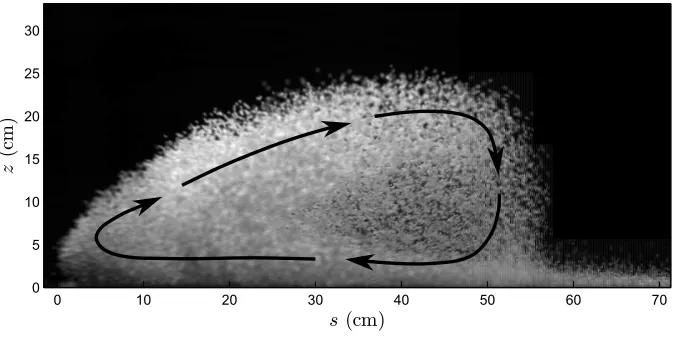
1.1. Flow features

It has been demonstrated both theoretically [16] and experimentally [20] that a gravity current head consists of a large rotating, vortex-like structure. The driving component of gravity accelerates the EPS beads and air downslope

towards the front of the flow. At the front of the flow this acceleration is

z

(c

m

)

s_(cm)

0 10 20 30 40 50 60 70

30

25

20

15

10

5

0

Figure 2: Side-on image of an EPS bead gravity current. sis the distance into the current

from the nose, where at the foremost point of the nose,s= 0. zis the perpendicular distance

from the chute surface, where at the chute surface, z = 0. Black arrows indicate relative

motion of EPS beads within the gravity current head.

−1 −0.5 0 0.5 1 1.5 2

−1 −0.8 −0.6 −0.4 −0.2 0 0.2 0.4 0.6 0.8 1

t(s)

p

(P

a)

Figure 3: A typical air pressure signal obtained from the chute surface of a laboratory scale

avalanche. The time origin,t= 0, corresponds to the time of maximum pressure when the

−0.5 0 0.5 1 1.5 −1.5

−1 −0.5 0 0.5 1 1.5

t

ψ

(

t

)

(a) Haar

0 0.5 1 1.5 2 2.5 3

−2 −1 0 1 2

t

ψ

(

t

)

(b) Daubechies type 2

0 5 10 15

−1 −0.5 0 0.5 1

t

ψ

(

t

)

(c) Daubechies type 10

−5 0 5

−0.5 0 0.5 1

t

ψ

(

t

)

(d) Mexican Hat

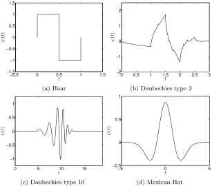
Figure 4: Examples of different types of wavelet function.

reaching the negative peak, the air behind the head becomes turbulent and the pressure returns to zero after the flow has passed.

1.2. Wavelet decomposition methods

This work makes use of a wavelet decomposition technique, to first de-noise and filter air pressure signals obtained from laboratory-scale PSAs, and then to visualize data and identify flow features. This technique was developed to be ap-plied to air pressure data signals, but is applicable to any other data time-series or one dimensional signal. Wavelet decomposition is a powerful technique that can be applied to many situations. Similar to Fourier-transform based tech-niques, time series data is transformed into the frequency domain. However, the advantage that a wavelet-based technique has over Fourier-transform based techniques is that time-domain information is retained during the transforma-tion. This makes it particularly useful in our context for filtering, de-noising and also identifying flow features. Wavelet-based techniques have also been shown to be a robust tool for surrogate data generation [11], which is a powerful technique in testing for nonlinearity in time series [19].

{

}

1.9 m

Electromagnet Mass

Adjustable pressure sensor mounting Air pressure

sensors

Release hopper

Variable slope angle,θ

1 m

Line release mechanism

0.85 m

z

y y

x

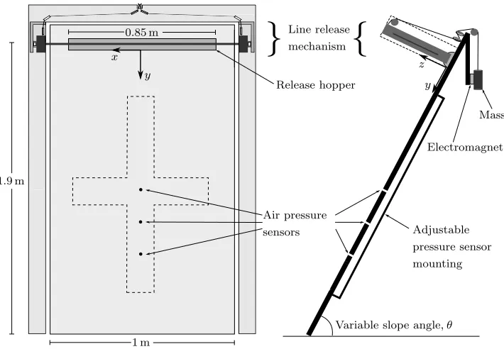
Figure 5: Front and side view schematic of the chute used for experiments.

duration that has an average value of zero. Unlike smooth and predictable sinu-soids, they tend to be irregular and asymmetric. Examples of various different types of wavelet function are shown in Figure 4.

Wavelets that have ‘sharp edges’ in the time domain (e.g. Haar (Figure 4(a)) or Daubechies type 2 (Figure 4(b))) have excellent temporal localization. This means that the properties of the signal at a point in time will correspond closely to the values for the wavelet coefficients at that point in time, with little smearing of the coefficients across neighbouring time positions. However, the frequency localization for this type of wavelet basis function is poor. Wavelets with higher numbers of vanishing moments (e.g. Daubechies type 10 (Figure 4(c)) or Mexican Hat (Figure 4(d))) have the opposite tendency, with good frequency localization and poor temporal localization [6].

The next section summarises the experimental setup where the air pressure signals were obtained. A more detailed description can be found in Jackson et al. [10].

2. Experimental set-up

The experiments were conducted on a 1 m wide, 1.9 m long, flat, open sided

wooden chute (Figure 5). The chute could be inclined at any angle between 60◦

and 90◦, where θ denotes the angle between the chute and the horizontal. To

create a pseudo two-dimensional line release, the lightweight granular material was released from a linear hopper which had a semi-elliptical cross section with

aspect ratio 0.9 and a length of 0.85 m.

The air flow in front of and inside the flows was measured using three cal-ibrated pressure transducers mounted in the surface of the chute (Figure 5). The pressure sensors used were Validyne DP 103 differential pressure trans-ducers with a range of 0 to 35 Pa. Similar to the experiments conducted by McElwaine and Nishimura [17], the sampling frequency of the sensors was set

at 1 kHz. Given the mean velocity of the flows,u≈2 m s−1_{, both the range and}

sampling rate of the pressure sensors are high enough to adequately capture the

flow features including any turbulent fluctuations (≈10u[20]).

To maximize the frequency response each of the sensors was connected to the

chute using a very short tube (≈40 mm) with resonant frequency approximately

2 kHz, which is significantly higher than the frequency of any features of the flow that we might expect to observe. The pressure sensors were connected to the same DAQ device as the electromagnet that controls the release mechanism, allowing acquisition of data from the pressure sensors to be synchronised with the release of the EPS beads.

The release mechanism was attached to a completely separate structure that surrounded the top and side edges of the chute. This meant that prior to release the only part of the mechanism that was in contact with the chute was the release hopper itself. As soon as the mechanism was operated all contact between the chute and the mechanism was broken (Figure 5), preventing vibrations being transmitted to the chute and affecting the readings from the sensitive pressure sensors attached to the chute.

In order to estimate the density of the EPS avalanche head, ρ, several

as-sumptions were necessary. The head of a fully suspended EPS avalanche is often modelled as being circular in cross section [2, 3, 21, 22]. Whist the heads formed in the EPS-air currents used in this work (Figure 2) are not semi-circular, the cross sectional area of the head is found to be approximately equal to that of a semi-circle with radius equal to the maximum height of the current

perpen-dicular to the plane of the chute hc. Therefore in order to calculate ρ, the

head of the current is assumed to be semi-circular in cross section, with radius

equal to the current head height, hc. The volume of the current can then be

approximated asVc = (πbh2c)/2 where b is the width of the release hopper. In

Figure 2 it can also be seen that some of the EPS beads are detrained from the rear of the head. Qualitatively the amount of material detrained from the rear was observed to be relatively small, and is difficult to accurately quantify as the

current progresses down the chute. Therefore, for the purpose of calculatingρ

it is also assumed that all of the EPS beads released are contained within the

current head, meaning that the proportion of Vc made up of EPS beads will

be equal to Vi. The proportion of Vc that is made up of entrained air is then

the current is then calculated asρ= [(1−V)ρa+V ρp], whereV =Vi/Vc.

3. Air pressure signal noise removal

3.1. Discrete Fourier Transform

Typical examples of signals obtained from one of the chute-mounted pressure sensors are shown in Figure 6. Whilst these signals display the features that we would expect to see for flows of this kind, namely a large positive pressure peak (Figure 6 - segment B) quickly followed by a negative peak (Figure 6 - segment C), the signals also contain a couple of features that are not related to the dy-namics of the flow. The first of these is low-amplitude, high-frequency electronic noise along the entire length of the signal (Figure 6 - segments A→D). The other

is a wave of peak amplitude approximately 0.5 Pa and frequency approximately

8 Hz that occurs during the first 0.75 s after the release mechanism is triggered

(Figure 6 - segment A). This is approximately the same amount of time that the release mechanism continued in motion for after the initial trigger, and is most likely to be caused by low-frequency pressure waves emitted by the sliding runners on the release mechanism being detected by the pressure sensors. The pressure signals therefore first need to be processed in order to remove these features before they can be used to study the dynamics of the flows.

Initially the signals were processed using a Fourier transform-based tech-nique. This involves transforming the signals from a time-domain

representa-tion to a frequency-domain representarepresenta-tion. For a pressure signalp(k) of length

Np this is achieved using a discrete Fourier transform (DFT), given by

P(j) = Np

X

k=1

p(k)ω(k_N−1)(j−1)

p (3)

where

ωN_p=e(−2πi)/Np ₍₄₎

is anNpth root of unity. In order to increase speed and efficiency the signals

are first zero padded so that their length is equal to a power of 2, this allows the implementation of a Fast Fourier transform (FFT) algorithm, reducing the

number of operations required fromN2

p to approximatelyNplog2(Np) [8]. The DFT of the signal is a complex number; the power in each frequency component represented by the DFT can be obtained by squaring the magnitude

of that frequency component. Thus, the power in thejth frequency component

is given by|P(j)|2_{. The power spectrum (Figure 7) obtained from the signal}

displayed in Figure 6b shows a peak at approximately 1 Hz which corresponds to the large positive and negative pressure peaks seen in the signal. Similar peaks were observed in the power spectra obtained from the other signals shown in Figure 6 (Appendix B.1). The signals also contain a wide range of higher

frequency (≈10−500 Hz) components whose power is close, but not equal, to

0 5 10 15 20 25 30 35 0

0.1 0.2 0.3 0.4 0.5

Frequency (Hz)

|

P

(

j

)

|

2

0 100 200 300 400 500

0 0.1 0.2 0.3 0.4 0.5

Frequency (Hz)

|

P

(

j

)

|

2

Figure 7: Single-sided power spectrum ofp(t) signal from an experiment with slope angle 80◦

wide range of frequencies involved, the power associated with each frequency component remains low. It can be deduced that the high frequency, low power components of the power spectrum shown in Figure 7 represent the electronic noise present in the signal. The power spectrum can therefore be used to filter out the electronic noise by identifying and removing the low power frequency components from the signal. This is achieved by setting a threshold power

level, Φ, and identifying the frequency components for which|P(j)|2_{<Φ. Once}

identified, these components are set to zero,P(j) = 0, and the inverse DFT,

p(k) = 1 Np

Np

X

j=1

P(j)ω_N−(k−1)(j−1)

p , (5)

is applied in order to convert the signal, with the low power frequency compo-nents removed, back into the time-domain.

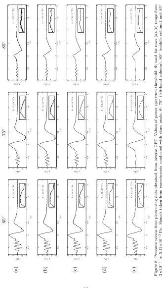
The effect on the output of the inverse DFT of applying different values of Φ to the power spectrum is shown in Figure 8, and it highlights the importance of selecting an appropriate value for Φ. Setting the value too low will mean that the electronic noise is not completely removed from the signal (Figure 8(a)). Whereas setting it too high will result in low power frequency components that are not necessarily electronic noise being removed from the signal (Figure 8(e)). It is reasonable to expect that the pressure signals obtained from the experi-ments will contain some higher frequency components arising from fluctuations in the flow caused by turbulence. The nature of the turbulence is such that these fluctuations are likely to be over short timescales and a wide range of frequen-cies and therefore, as with electronic noise, the power levels of these frequency components will be low. A drawback of using a DFT-based filtering technique to remove electronic noise is that it is extremely difficult to identify which of the lower power frequency components relate to noise and which relate to genuine flow features, and set an appropriate value of Φ accordingly. Another drawback

of this technique is that in order to remove the≈8 Hz wave in the early part of

the signal the value of Φ needs to be relatively high. This also results in features with the same frequency, and frequencies with the same or lower power levels, that occur later in the signal being filtered out.

Applying a power-level based threshold in the frequency domain is not the only available method of filtering using the DFT of a signal. A frequency-level based threshold whereby any frequencies above a certain value are removed can also be applied to the output of the DFT. Whilst this avoids the problem of unwanted removal of low-power, low-frequency signal features, the problem of setting a threshold that retains low-power, higher frequency signal features while removing unwanted electronic noise still remains.

3.2. Wavelet analysis

signal. Therefore if in addition to frequency and power, time information was also available, electronic noise would be easily identifiable as the low power, high frequency components that occur at all points in time along the signal. This is in contrast to other high-frequency components, such as those relating to turbulence, that only occur at certain periods of time along the signal. Simi-larly, time information could be used to easily remove the pressure wave at the

beginning of the signal by identifying all of the frequency components of≈8 Hz

that occur during the first 0.75 s of the signal.

Attempts can be made to address these drawbacks by adapting the Fourier transform to analyse only a small section, or window, of the signal at a time. The short-time Fourier transform (STFT), maps a signal into a two-dimensional function of time and frequency, providing a compromise between the time- and frequency-based views of the signal. Different values of Φ could then be applied when filtering different parts of the signal. However, the information about when and at what frequencies a signal feature occurs at can only be obtained with limited precision, and that precision is determined by the size of the window [1]. Once a particular size for the time window has been chosen, that window is the same for all frequencies. A more flexible approach is required where the window size can be varied in order to determine more accurately time or frequency data relating to signal features.

This more flexible approach exists in the form of wavelet analysis. Wavelet analysis allows the use of long time intervals where more precise low-frequency is required, and shorter regions where high-frequency information is required [14].

Wavelet analysis is performed by the translation and dilation of the mother wavelet along a signal and the convolution of this function with the signal. The

continuous wavelet transform (CWT) for a signalpthat varies with timetbased

on a mother waveletψis given by

CW T(j, k) = √1 j

Z +∞

−∞ p(t)ψ

_t−k

j

dt, (6)

wherejandkare the dilation and translation parameters of the mother wavelet

ψ. If the length of the signal isNp, the CWT producesNpcoefficients at every

scale analysed. The wavelet basis function used here is a Daubechies wavelet with 5 vanishing moments (Figure 9, described mathematically in Daubechies [6] chapter 6), which was selected as a good compromise between time and frequency localization. This is suitable since the signals contain a wide range of a wide range of time variant frequencies (Figure 6).

Wavelet analysis can be performed more efficiently by replacing the CWT with the discrete wavelet transform (DWT). In this case, the dilation is per-formed in powers of two, with the mother wavelet starting at its minimum

width and is doubled at each dyadic scale j. The DWT is calculated using a

hierarchical cascade of filter banks, making it more efficient numerically, while dramatically reducing the number of wavelet coefficients produced.

The DWT of a time series sampled at Np = 2j _{points can be formulated}

0 1 2 3 4 5 6 7 8 9 −1.5

−1 −0.5 0 0.5 1 1.5

t

ψ

(

t

)

quadrature mirror filters of even filter width, Λ, wherehl(l = 0, . . . ,Λ−1) is

the high pass (or wavelet) filter,gl is the low pass (or scaling) filter and

gl≡(−1)l+1hΛ−1−l (7)

At the first stage of the algorithm,j= 1, these filters are circularly convolved

withp(t) and the downsampled by a factor of 2 to give a set of wavelet,w, and

approximation,A, coefficients of lengthNp/2:

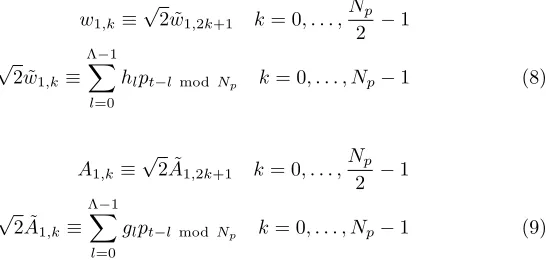
w1,k≡√2 ˜w1,2k+1 k= 0, . . . ,Np

2 −1

√

2 ˜w1,k≡ Λ−1 X

l=0

hlpt−l modNp k= 0, . . . , Np−1 (8)

A1,k≡√2 ˜A1,2k+1 k= 0, . . . ,Np

2 −1

√

2 ˜A1,k≡ Λ−1 X

l=0

glpt−lmodNp k= 0, . . . , Np−1 (9)

At subsequent stages of the algorithm,j, the approximation from the previous

stage of the algorithm,Aj−1,k is used instead of p(t) in Equations 8 and 9 to

give wavelet coefficients over all scalesj = 1, . . . , J and a final approximation

coefficient.

A drawback of the DWT is that as the scale doubles, the number of wavelet coefficients halves, which makes comparative analysis between scales problem-atic. Therefore the stationary wavelet transform (SWT) is instead used, which retains the efficiency of working with dyadic scales only but is an undecimated transform, as the downsampling undertaken in the DWT is eliminated. This means that each point in time has a unique coefficient for each scale, i.e. there

are Np wavelet coefficients at each scale, making between-scale analysis

eas-ier. A detailed description of the implementation of the SWT can be found in Appendix A.

A minor drawback of the SWT is that 2j has to be a factor of the length of

the signal,Np, forj= 1, . . . , J. However, this can be overcome in this situation

by extending the signal up to the next dyadic scale using zero padding at the end of the signal. The fact that the signal already starts and finishes with values of approximately zero, the addition of zero padding does not cause any significant discontinuities in the signal that may affect the SWT, and the padding can be removed after the filtering has been performed.

Figure 10 shows the output of multiscale SWT when applied to the pressure signal shown in Figure 6(b). The signal has been decomposed into

approxima-tion coefficients at scale j = 7 and wavelet coefficients at scalesj = 1, . . . ,7.

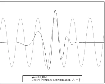
Wavelet Db5

Centre frequency approximation,F_c=2 3

Scale, Pseudo-frequency,

j Fj (Hz)

1 333

2 167

3 83

4 41

5 21

6 10

7 5

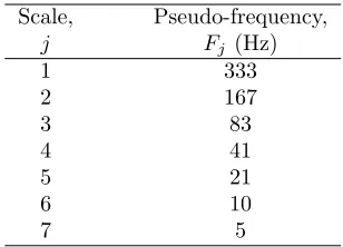
Table 1: Wavelet scales and their equivalent pseudo-frequencies.

a purely periodic signal of frequency Fc (Figure 11), known as the centre

fre-quency.Fcis equal to the frequency that maximises the fast Fourier transform of

the wavelet modulus, which for the Db5 wavelet is 2₃Hz. The pseudo-frequency,

Fj, in Hz is then given by

Fj = Fc

j·∆, (10)

where j is the scale and ∆ is the sampling period. The pseudo-frequencies

corresponding to the wavelet scales from the SWT decomposition in Figure 10 are shown in Table 1.

Looking at the multiscale SWT decomposition of the pressure signal (Fig-ure 10), it can be seen that the high-frequency components of the signal that

are filtered into wavelet scales w1,k and w2,k are rapidly fluctuating but with

approximately constant magnitude throughout the entire length of the signal

Np. Wavelet scalesw3,k,w4,kand w5,k also contain some low-amplitude,

time-invariant components. Similar features were observed in the multiscale SWT decompositions of other signals (shown in Figure 6 and Appendix B.2). The fact that the components are high-frequency, time-invariant and present throughout the entire length of the signals, suggests that they correspond to the effects of electronic noise on the signal.

It is likely that there will be various forms of electronic noise present in the signals obtained from the pressure sensing equipment. This electronic noise is approximately white, with power spectral density nearly constant throughout the frequency spectrum and its amplitude will have very nearly a Gaussian

prob-ability density function. The mean value of the wavelet scalew1,k coefficients

is approximately zero and they follow an approximately Gaussian distribution (Figure 12), so it is therefore assumed that they correspond to the electronic noise present in the signal. This wavelet scale is therefore used to set a thresh-old value for filtering out the electronic noise from the signal. The threshthresh-old

value is obtained using estimates of the wavelet scalew1,k coefficients’ standard

−0.01 −0.008 −0.006 −0.004 −0.002 0 0.002 0.004 0.006 0.008 0.01 0

20 40 60 80 100 120 140 160 180 200

Coefficient value

F

re

q

u

en

cy

(a)

−0.01 −0.008 −0.006 −0.004 −0.002 0 0.002 0.004 0.006 0.008 0.01

0 50 100 150 200 250 300 350

Coefficient value

F

re

q

u

en

cy

(b)

Figure 12: Histogram of wavelet scalew1,k coefficient values (grey bars) corresponding to

electronic noise for (a) data from an experiment with slope angle 80◦ and (b) combined

data from three experiments with slope angles 75◦_{, 80}◦_{and 85}◦_{. Black line shows a normal}

applied to the wavelet scalew1,kcoefficients in order to determine the threshold value.

Once the threshold value has been obtained it is applied to all the wavelet scales, but not the approximation coefficients, and coefficients with magnitude less than the threshold value are set to zero (Figure 13). The de-noised signal and residuals (calculated by subtracting the de-noised signal from the original

signal) are shown in Figure 14. The mean value of the residuals, ¯R, is

approxi-mately zero and the approxiapproxi-mately constant level of variation across the entire length of the signal, indicate that the wavelet coefficients of the signal removed during the de-noising process correspond only to the electronic noise present in the signal and that no other signal features have been lost. This thresholding technique was also applied to the multiscale SWT decompositions obtained from the other two signals in Figure 6(a) and (c). The results of which are shown in Appendix B.3 and demonstrate that the technique is also effective in removing white noise from other signals.

Attention is now turned to the removal of the low-frequency pressure waves that appear at the beginning of the signal. Conversely to the electronic noise, the bulk of the coefficients that correspond to these pressure waves are found

in wavelet scales w7,k and w6,k, and a minority are found in wavelet scales

w5,k,w4,kandw3,k (Figure 10). This is to be expected as, as previously noted,

the pressure wave has a frequency of ≈8 Hz and wavelet scalesw7,k and w6,k

correspond to a frequency range of≈5 - 10 Hz. The fact that the effects of the

pressure wave are only observed during the early part of the signal means that

the wavelet scales can be split by introducing an interval at a certain value oft

(ork), and filtering only applied to pre-interval wavelet coefficients.

A wavelet coefficient variance or autocorrelation based technique could be used in order to identify coefficients that correspond to the unwanted part of the signal (i.e. the soundwave) and then remove them. This would then give the advantage of being able to remove unwanted periodic signal elements no matter whereabouts they occur in the signal.

While sophisticated automated interval identification algorithms do exist [7, 13, 23], scrutinisation of a large number of pressure signals revealed that

the pressure wave consistently occurred during the first 0.75 s of the signal,

additionally the earliest positive pressure peaks caused by the current arriving at

the first (lowest value ofs) sensor occurred at≈0.85 s. Given these observations,

coupled with the fact the main aim of studying these pressure signals is to gain information about the internal dynamics of the currents (i.e. from the positive pressure peak and onwards), use of automated interval identification algorithms was deemed unnecessary, and instead a fixed interval separation point was placed

at 0.75 s (or k = 750) for all wavelet scales. All wavelet coefficients occurring

0 500 1000 1500 2000 2500 3000 −1

−0.5 0 0.5 1

Original signal,p(k)

k

p

(P

a)

(a)

0 500 1000 1500 2000 2500 3000

−1 −0.5 0 0.5 1

De-noised signal,Dp(k)

k

p

(P

a)

(b)

0 500 1000 1500 2000 2500 3000

−0.01 −0.005 0 0.005

0.01 Residuals

k

p

(

k

)

−

Dp

(

k

) R¯= 6.7 x 10

−6

(c)

0 500 1000 1500 2000 2500 3000 −1

−0.5 0 0.5 1

De-noised signal,Dp(k)

k

p

(P

a)

(a)

0 500 1000 1500 2000 2500 3000

−1 −0.5 0 0.5 1

Interval-filtered signal,Fp(k)

k

p

(P

a)

(b)

0 500 1000 1500 2000 2500 3000

−0.2 −0.1 0 0.1

0.2 Residuals

k Dp

(

k

)

−

Fp

(

k

)

(c)

demonstrate that this technique was also effective when applied to other signals.

4. Wavelet-based visualisation of air pressure signal features

An additional advantage of using the wavelet-based method for de-noising of the signals is that it forms the basis of, and can easily be extended to, a method for visualization of a signal’s features developed by Keylock [12]. This technique makes use of the wavelet decomposition data and allows wavelet coefficients and scales that actively contribute to flow features to be identified. In order to achieve this the variance of the wavelet coefficients, both on a global and scale-by-scale level, is first calculated. All wavelet coefficients are set to zero where the sign of the coefficient at a point in time is opposite that of the sum of the coefficients at that point in time. The remaining coefficients are then normalised by the global (Figure 17(b)) or scale-by-scale (Figure 17(c)) standard deviations for each component.

The advantage of this method over a standard SWT decomposition, is that only wavelet coefficients that contribute to a particular flow event are shaded, since coefficients with an opposite sign are in white. This makes it easier to focus upon the relevant scales for generating a particular flow event and hence the likely processes in operation. Scaling with respect to the global variance indicates the scales that dominate the whole flow (Figure 17(b)), but makes it harder to determine the importance of a contribution at a particular scale to the detected flow event. Normalising with respect to scale-by-scale variances (Figure 17(c)) compensates for differences in energy between scales and produces a wavelet spectrum analogous to the Fourier spectrum. It can be seen in Figure 17(b) that overall the flow is dominated by the high amount of energy at level 7,

correlating with the peak at≈1 Hz in the power spectrum produced from the

DFT of the signal. This energy corresponds to the large positive and negative pressure peaks caused by the large vortex-like structure at the centre of the flow. However when differences in energy between scales are accounted for, it is found that higher frequency (scales 2–6) components that occur around and after the negative pressure peak are equally significant (Figure 17(c)). It seems likely that these high frequency components correspond to fluctuations in the flow velocity caused by turbulence.

De-noised and filtered pressure signals from a series of experiments with the same release volume, EPS bead diameter and slope angle have been superim-posed in Figure 18(a). The low frequency signal features are highly repeatable and are well represented by the ensemble average signal (RMS residual from

ensemble mean = 3.3×10−2_{)(Figure 18(b)). However information about the}

−0.5 0 0.5 1 1.5 2

−0.6 −0.4 −0.2 0 0.2 0.4 0.6

t(s)

p

(P

a)

(a)

W

a

v

e

le

t

S

c

al

e

1

2

3

4

5

6

7

(b)

W

a

v

e

le

t

S

c

al

e

1

2

3

4

5

6

7

(c)

−1 −0.5 0 0.5 1 1.5 2 −1.5

−1 −0.5 0 0.5 1 1.5

t(s)

p

(P

a)

(a)

−1 −0.5 0 0.5 1 1.5 2

−1.5 −1 −0.5 0 0.5 1 1.5

t(s)

p

(P

a)

(b)

Figure 18: (a) Air pressure signals from five 3300 cm3_{of 2.7 mm diameter EPS bead currents}

at a slope angle of 80◦. (b) Ensemble mean of signals shown in (a) (solid line) plus or minus

W

av

el

et

S

cal

e

t_(s)

−0.5 0 0.5 1 1.5 2

1

2

3

4

5

6

7

Figure 19: Ensemble wavelet-based visualisation of flow features. Wavelet coefficients

nor-malised by scale-by-scale wavelet variance. Darker values indicate a higher value for the

coefficients and coefficients that are opposite in sign to the detected fluctuation are set to zero.

obtained. The wavelet coefficient data collected from each individual experi-ment can then be used to produce an ensemble of all the experiexperi-ments conducted (Figure 19), and general trends in the scale and occurrence of flow features iden-tified.

5. Conclusions

Wavelet-based analysis techniques have been demonstrated to be an ex-tremely useful tool for processing and studying air pressure signals obtained from laboratory-scale PSAs. As well as de-noising and filtering the signals, wavelet-based analysis has been demonstrated to be capable of enabling visu-alisation of flow data and identification of important flow events. Information about both the time and frequency levels of these events can be obtained as well as their energy levels relative to both the energy of other events with similar frequencies and to the total energy of the signal as a whole. In addition to being applied to data obtained from laboratory-scale experiments, these wavelet-based techniques could also be applied to field or large-scale model PSA air pressure data, or indeed any other kind of time series data.

Appendix A. The Stationary Wavelet Transform

In order to implement the stationary wavelet transform (SWT), the filters first need to be rescaled to account for the lack of downsampling. Defining the

filter width at scalej as Λj≡(2j−1)(Λ−1) + 1, thejth level SWT high and

low pass filters are expressed as

˜

hj,l ≡hj,l/2j/2

˜

gj,l≡gj,l/2j/2. (A.1)

The SWT wavelet and approximation coefficients (equivalent to the DWT ex-pressions in Equations 8 and 9) are then given as

wj,k≡ Λi−1

X

l=0 ˜

hj,lpk−l modNp

Aj,k≡ Λi−1

X

l=0 ˜

gj,lpk−l modNp. (A.2)

The filters then require periodization so that, instead of an explicit circu-lar convolution with Equation A.1, implicit circucircu-lar filtering using a standard convolution and a periodized filter is performed, where

˜ h◦_j,l≡

+∞ X

n=−∞

˜

hj,l+nNp. (A.3)

Expressing Equation A.2 in terms of Equation A.3 gives

w◦_j,k≡ Np−1

X

l=0 ˜

h◦_j,lpk−lmodNp

A◦_j,k≡ Np−1

X

l=0 ˜

0 5 10 15 20 25 30 35 0

0.05 0.1 0.15 0.2 0.25 0.3 0.35 0.4

Frequency (Hz)

|

P

(

j

)

|

2

0 100 200 300 400 500

0 0.05 0.1 0.15 0.2 0.25 0.3 0.35 0.4

Frequency (Hz)

|

P

(

j

)

|

2

Figure B.20: Single-sided power spectra ofp(t) signal from an experiment with slope angle

75◦(e.g. Figure 6(a)), main: x-axis shortened for clarity, inset: fullx-axis shown.

Equation A.4 can then be evaluated from a recursion which states that, given

the approximationA◦_j,k,w◦_j+1,kand A◦_j+1,k can be obtained from

w◦j+1,k = Λ−1 X

l=0 ˜

h◦lA◦j,k−2j_lmodNp

A◦_j+1,k= Λ−1 X

l=0 ˜

g_l◦A◦_j,k−2j_lmodNp (A.5)

Appendix B. Wavelet Analysis of Other Pressure Signals

Appendix B.1. Power Spectra of Pressure Signals

Power spectra obtained from the DFT of the pressure signals from

experi-ments with slope angles 75◦ (e.g. Figure 6(a)) and 85◦ (e.g. Figure 6(c)) are

0 5 10 15 20 25 30 35 0

0.05 0.1 0.15 0.2 0.25

Frequency (Hz)

|

P

(

j

)

|

2

0 100 200 300 400 500

0 0.05 0.1 0.15 0.2 0.25

Frequency (Hz)

|

P

(

j

)

|

2

Figure B.21: Single-sided power spectra ofp(t) from an experiment with slope angle 85◦_(e.g.

Appendix B.2. Multiscale SWT Decomposition of Pressure Signals

Multiscale SWT decompositions of the pressure signals from experiments

with slope angles 75◦ (e.g. Figure 6(a)) and 85◦(e.g. Figure 6(c)) are shown in

Figures B.22 and B.23 respectively.

Appendix B.3. De-noised Pressure Signals

Wavelet coefficients and de-noising threshold levels of the pressure signals

from experiments with slope angles 75◦(e.g. Figure 6(a)) and 85◦ (e.g. Figure

6(c)) are shown in Figure B.24. The original signals, de-noised signals and residuals of the de-noised signals are shown in Figure B.25.

Appendix B.4. Interval-filtered Pressure Signals

Wavelet coefficients and filtering intervals of the pressure signals from

ex-periments with slope angles 75◦ (e.g. Figure 6(a)) and 85◦ (e.g. Figure 6(c))

are shown in Figure B.26. The de-noised signals, interval-filtered signals and residuals of the filtered signals are shown in Figure B.27.

[1] Allen, J. B., 1977. Short time spectral analysis, synthesis, and modification by discrete Fourier transform. IEEE Transcations on Acoustics, Speech, and Signal Processing 25 (3), 235–238.

[2] Batchelor, G. K., 1967. An Introduction to Fluid Mechanics. Cambridge University Press, Cambridge, UK.

[3] Beghin, P., Brugnot, G., 1983. Contribution of theoretical and experimen-tal results to powder-snow avalanche dynamics. Cold Regions Science and Technology 8, 63–73.

[4] Birge, L., Massart, P., 1997. Festschrift for Lucien Le Cam. Research Papers in Probability and Statistics. Springer, New York, Ch. From model selection to adaptive estimation, pp. 55–87.

[5] Bozhinskiy, A. N., Sukhanov, L., 1998. Physical modelling of avalanches using an aerosol cloud of powder material. Annals of Glaciology 26, 242– 394.

[6] Daubechies, I., 1992. Ten Lectures on Wavelets. CBMS-NSF Regional Con-ference Series in Applied Mathematics. Society for Industrial and Applied Mathematics.

[7] Donoho, D. L., Johnstone, I. M., 1994. Ideal spatial adaptation by wavelet shrinkage. Biometrika 81, 425–455.

[8] Duhamel, P., Vetterli, M., 1990. Fast Fourier transforms: A tutorial review and a state of the art. Signal Processing 19, 259–299.

0 1000 2000 3000 −0.01

0 0.01

k

w1

−0.02 0 0.02

w2

−0.05 0 0.05

w3

−0.1 0 0.1

w4

−0.2 0 0.2

w5

−2 0 2

w6

−2 0 2

De-noised wavelet coe_fficients

w7

0 1000 2000 3000

−0.01 0 0.01

k

w1

−0.02 0 0.02

w2

−0.05 0 0.05

w3

−0.1 0 0.1

w4

−0.2 0 0.2

w5

−2 0 2

w6

−2 0 2

Wavelet coe_fficients

w7

(a)

0 1000 2000 3000

−0.01 0 0.01

k

w1

−0.01 0 0.01

w2

−0.02 0 0.02

w3

−0.05 0 0.05

w4

−0.1 0 0.1

w5

−1 0 1

w6

−1 0 1

De-noised wavelet coe_fficients

w7

0 1000 2000 3000

−0.01 0 0.01

k

w1

−0.01 0 0.01

w2

−0.02 0 0.02

w3

−0.05 0 0.05

w4

−0.1 0 0.1

w5

−1 0 1

w6

−1 0 1

Wavelet coe_fficients

w7

(b)

Figure B.24: Original (left hand column) and de-noised (right hand column) wavelet

coeffi-cients at all scales for pressure signals from experiments with slope angle: (a) 75◦(e.g. Figure

0 1000 2000 3000 −0.02

0 0.02

k

w1

−0.02 0 0.02

w2 −0.05

0 0.05

w3

−0.1 0 0.1

w4

−0.2 0 0.2

w5

−1 0 1 w6

−2 0 2

Interval-_filtered wavelet coe_fficients

w7

0 1000 2000 3000

−0.02 0 0.02

k

w1

−0.02 0 0.02

w2 −0.05

0 0.05

w3

−0.1 0 0.1

w4

−0.2 0 0.2

w5

−1 0 1 w6

−2 0 2

De-noised wavelet coe_fficients

w7

(a)

0 1000 2000 3000

−0.02 0 0.02

k w1

−0.02 0 0.02

w2

−0.05 0 0.05

w3

−0.1 0 0.1

w4

−0.2 0 0.2

w5 −1

0 1

w6

−1 0 1

Interval-_filtered wavelet coe_fficients

w7

0 1000 2000 3000

−0.02 0 0.02

k w1

−0.02 0 0.02

w2

−0.05 0 0.05

w3

−0.1 0 0.1

w4

−0.2 0 0.2

w5 −1

0 1

w6

−1 0 1

De-noised wavelet coe_fficients

w7

(b)

Figure B.26: De-noised (left hand column) and interval-filtered (right hand column) wavelet

coefficients at all scales for pressure signals from experiments with slope angle: (a) 75◦(e.g.

Figure 6(a)) and (b) 85◦(e.g. Figure 6(c)). Black dashed lines indicate the interval separation

[10] Jackson, A., Turnbull, B., Munro, R., 2013. Scaling for lobe and cleft pat-terns in particle-laden gravity currents. Nonlinear Processes in Geophysics 20, 121–130.

[11] Keylock, C., 2007. A wavelet-based method for surrogate data generation. Physica D 225, 219–228.

[12] Keylock, C. J., 2007. The visualization of turbulence data using a wavelet-based method. Earth Surface Processes and Landforms 32, 637–647.

[13] Lavielle, M., 1999. Detection of multiple changes in a sequence of dependent variables. Stochastic Processes and their Applications 83, 79–102.

[14] Mallat, S., 1998. A Wavelet Tour of Signal Processing. Academic Press.

[15] Massey, B. S., 2006. Mechanics of Fluids, 8th Edition. Taylor & Francis, Abingdon, UK.

[16] McElwaine, J. N., 2004. Rotational flow in gravity current heads. Philo-sophical Transactions of the Royal Society 363, 1603–1623.

[17] McElwaine, J. N., Nishimura, K., 2001. Particulate Gravity Currents. Vol. 31 of Special Publication of the International Association of Sedimen-tologists. Blackwell Science, Malden, Massachusetts, USA, Ch. Ping-pong Ball Avalanche Experiments, pp. 135–148.

[18] Nohguchi, Y., Ozawa, H., 2008. On the vortex formation at the moving front of lightweight granular particles. Physica D 238, 20–26, doi:10.1016/j.physd.2008.08.019.

[19] Theiler, J., Eubank, S., Longtin, A., Galdrikian, B., Farmer, J., 1992. Test-ing for nonlinearity in time series: the method of surrogate data. Physica D 58, 77–94.

[20] Turnbull, B., McElwaine, J. N., 2008. Experiments on the non-Boussineq flow of self-igniting suspension currents on a steep open slope. Journal of Geophysical Research 113 (F01003), doi:10.1029/2007JF000753.

[21] Turnbull, B., McElwaine, J. N., 2010. Potential flow models of suspension current air pressure. Annals of Glaciology. 51 (54).

[22] Turnbull, B., McElwaine, J. N., Ancey, C., 2007. Kulikovskiy-Sveshnikova-Beghin model of powder snow avalanches: Development and application. Journal of Geophysical Research 112 (F01004), doi:10.1029/2006JF000489.