An SPH multi fluid model based on quasi buoyancy for interface stabilization up to high density ratios and realistic wave speed ratios

DOI: 10.1002/fld.4498

R E S E A R C H A R T I C L E

An SPH multi-fluid model based on quasi buoyancy for

interface stabilization up to high density ratios and realistic

wave speed ratios

A.C.H. Kruisbrink

_{F.R. Pearce}

_{T. Yue}

_{H.P. Morvan}

1_{Gas Turbine Transmissions Research}

Centre, University of Nottingham, Nottingham, UK

2_{School of Physics and Astronomy,}

University of Nottingham, Nottingham, UK

Correspondence

A.C.H. Kruisbrink, Gas Turbine Transmissions Research Centre, University of Nottingham, Nottingham, NG7 2RD, United Kingdom.

Email:

[email protected]

Funding information

Rolls-Royce and the European Union within the research project ELUBSYS (Engine Lubrication System

Technologies), Grant/Award Number: ACP8-GA-2009-233651

Summary

We introduce a smoothed particle hydrodynamics (SPH) concept for the stabi-lization of the interface between 2 fluids. It is demonstrated that the change in the pressure gradient across the interface leads to a force imbalance. This force imbalance is attributed to the particle approximation implicit to SPH. To stabi-lize the interface, a pressure gradient correction is proposed. In this approach, the multi-fluid pressure gradients are related to the (gravitational and fluid) accelerations. This leads to a quasi-buoyancy correction for hydrostatic (strat-ified) flows, which is extended to nonhydrostatic flows. The result is a simple density correction that involves no parameters or coefficients. This correction is included as an extra term in the SPH momentum equation. The new concept for the stabilization of the interface is explored in 5 case studies and compared with other multi-fluid models. The first case is the stagnant flow in a tank: The interface remains stable up to density ratios of 1:1000 (typical for water and air), in combination with artificial wave speed ratios up to 1:4. The second and third cases are the Rayleigh-Taylor instability and the rising bubble, where a reason-able agreement between SPH and level-set models is achieved. The fourth case is an air flow across a water surface up to density ratios of 1:100, artificial wave speed ratios of 1:4, and high air velocities. The fifth case is about the propagation of internal gravity waves up to density ratios of 1:100 and artificial wave speed ratios of 1:2. It is demonstrated that the quasi-buoyancy model may be used to stabilize the interface between 2 fluids up to high density ratios, with real (low) viscosities and more realistic wave speed ratios than achieved by other weakly compressible SPH multi-fluid models. Real wave speed ratios can be achieved as long as the fluid velocities are not very high. Although the wave speeds may be artificial in many cases, correct and realistic wave speed ratios are essential in the modelling of heat transfer between 2 fluids (eg, in engineering applications such as gas turbines).

K E Y WO R D S

interface treatment, multi-fluid, smoothed particle hydrodynamics

1

I N T RO D U CT I O N

Many real-world fluid flow problems involve more than one fluid, with the physical outcome differing significantly if we include air rather than vacuum in the model. Pipe-filling and emptying and fluid break-up are only 2 amongst many

. . . . This is an open access article under the terms of the Creative Commons Attribution-NonCommercial License, which permits use, distribution and reproduction in any medium, provided the original work is properly cited and is not used for commercial purposes.

Copyright © 2018 The AuthorsInternational Journal for Numerical Methods in FluidsPublished by John Wiley & Sons Ltd.

possible examples. In the case of liquid-gas flows, the density ratio between the 2 fluids is usually very high, eg, for water-air flow under atmospheric conditions, the density ratio is around 800.

Several multi-fluid models are available in the literature for incompressible fluids (eg, see the works of Cummins and Rudman,1 _{Hu and Adams,}2,3_{and Xu et al}4_{) as well as for weakly compressible fluids, where this paper focuses on. The} most important multi-fluid models in the literature and their main features are described below.

Ritchie and Thomas5_{suggested a summation of the particle-averaged pressure (instead of density), to deal with steep} density gradients. This effectively creates smoothedpressurehydrodynamics. The main drawbacks of their method are difficulties in the treatment of shocks and the need to follow the internal energy.

Colagrossi and Landrini6 _{used a density renormalization at intermediate time steps, a large artificial surface tension} and a high wave speed for the low-density fluid, and a smoothing of the velocity field. In addition to these unphysical aspects, very small time steps are required.

Flebbe et al7_{introduced the “particle number density” approach of smoothed particle hydrodynamics (SPH) to} astro-physics. Ott and Schnetter8 _{and Hu and Adams}9 _{applied it to fluid engineering to estimate the density of multi-fluids.} Following on from this work, Colagrossi et al10_{applied it to develop an equation of motion for multi-fluids. The main} restriction of this method is that the particle volume (V) and the change of volume (ΔV/V) due to compression must remain the same for different fluids. The latter means that the choice of the wave speed ratio is rather limited, usually resulting in a higher wave speed for the lower-density fluid. For air and water with a density ratio of 1:1000, a wave speed ratio of 14:1 would be required. Another restriction is that the method, usually based on a standard SPH density estimate (ie, in the summation form), cannot be applied to free-surface flows.

Adami et al11_{also applied the particle number density to the equation of motion. They use a (density-weighted) average} pressure to deal with the pressure gradient across the interface. This leads to a better estimate of the pressure gradient but does not guarantee a stable interface, in particular, at high density ratios.

Grenier et al12_{used a density renormalization with a variant of the Shepard correction, in which the particle volume is} obtained from the continuity equation. In addition, they use a repulsive force between particles of different fluids similar to that suggested by Monaghan13_{to stabilize the interface.}

Monaghan and Rafiee14_{used the continuity equation in a form suited to multi-fluid flows. They also use a repulsive} force to stabilize the interface between 2 fluids similar to that for the tensile instability suggested by Monaghan13 _and to that used by Grenier et al.12_{The concept is applied to high density ratios up to 1000. However, the wave speed of the} low-density fluid (gas) is still a factor 5 to 7 higher than that of the high-density fluid (liquid).

Khayyer et al15_{introduced an incompressible-compressible moving particle semi-implicit method. The 2 phases are} modeled with incompressible and compressible forms of the pressure Poisson equation, which are solved with projection methods. The method suffers from numerical errors in volume conservation, which are reduced by using compensating terms, to keep the density variations within an allowable range. To allow for high density ratios, a smoothing of the density discontinuity across the interface is required.16

Lind et al17,18_{introduced an incompressible-compressible SPH method, where incompressible SPH and weakly} com-pressible SPH (WCSPH) are coupled. The incomcom-pressible phase provides the velocity, and the comcom-pressible phase provides the pressure as the boundary condition for the other phase at the interface. The method is applied to high density ratios of 1:1000. It allows for real wave speeds of the compressible phase. Further artificial viscosity is used in the compressible phase for numerical stabilization, and (Fickian) particle shifting in the incompressible phase to avoid particle clustering. The application of the aforementioned multi-fluid models for weakly compressible SPH is limited by density ratios and/or wave speed ratios. The models in the works11,12,14_{deal to some extend with the particle instability caused by the} change of the pressure gradient across the interface. In this paper, we aim for water-air applications with density ratios up to 1000, physically real viscosities, and realistic wave speed ratios. For this purpose, a novel WCSPH multi-fluid model based on a density correction is introduced.

2

PA RT I C L E I N STA B I L I T Y AT I N T E R FAC E

2.1

SPH particle approximation

because of body forces (principally gravitation but also inertia associated with fluid accelerations), there is a discontinuity in the pressure gradient.

According to the SPH particle approximation, the value of a property associated with particleiis evaluated from a convolution summation over its neighbour particlesj

⟨

𝑓(xi⃗)⟩=∑

𝑗

𝑓(x⃗_𝑗)V_𝑗W_𝑖𝑗, (1)

wherefis a generic field function,Vis the particle volume, andWij=W(|xi–xj|,h) is a weighting or kernel function bounded by the smoothing lengthh. The consequence of the particle approximation with its weighted volume summation is that surface forces at the interface are smoothed and treated as body forces near the interface. Because of the discon-tinuity in the pressure gradient, the pressure forces on particles near the interface are no longer balanced, leading to a particle instability. This is demonstrated in the next subsections by considering 2 cases: a stagnant stratified flow and a more general accelerating flow.

2.2

Stagnant flow

Consider a fluid column consisting of 2 stagnant fluidsαandβ. As illustrated in Figure 1, the pressure distribution within the 2 stratified fluid layers is hydrostatic. The pressure gradient changes at the interface due to the density difference.

In the continuum limit, the fluid around the interface is at rest because of the equilibrium of the surface forces. However, because SPH particles are modeled discretely by smoothed body forces, the fluid particles near the interface are not at rest. As illustrated in Figure 1, particleifeels the higher pressure of neighbour particlej, which resides in the other fluid. This excess pressure will tend to move it upwards. It would stay at rest if its hydrostatic pressure distribution was extrapolated (as shown in Figure 1 by the dotted line on the right-hand panel) within the kernel support domain (yellow circle on the left-hand panel).

The particle instability is revealed by unphysical particle motions, which is demonstrated in the first case study: “stagnant flow in tank” in Section 5.1.

2.3

Accelerating flow

Now, consider a fluid column consisting of 2 fluidsαandβ, which is uniformly accelerated in the absence of gravity. For a continuum fluid, the “kinematic” boundary conditions at the interface, in the absence of surface tension, are

v_𝛼=v_𝛽 ; 𝑝𝛼 =𝑝𝛽 ; 𝜏𝛼 = − 𝜏𝛽. (2)

FIGURE 1 Stagnant stratified flow. Left: red and blue particles represent 2 different fluids near an interface, with the lighter fluid (blue) on top of the denser fluid (red). Gravity is assumed to act vertically downwards. The yellow circle indicates the SPH kernel support domain of

particlei. The kernel of this particle extends over the interface between the fluids. Right: the hydrostatic pressure distribution within the 2

For inviscid fluids, it follows from the Euler equations that 1

𝜌𝛼 𝜕𝑝𝛼

𝜕n = − dvn,𝛼

dt ;

1

𝜌𝛽 𝜕𝑝𝛽

𝜕n = − dvn_,𝛽

dt . (3)

Combining the previous equations yields for the “dynamic” boundary conditions

dvn_,𝛼 dt =

dv_n,𝛽

dt ⇒

1

𝜌𝛼 𝜕𝑝𝛼

𝜕n = 1

𝜌𝛽 𝜕𝑝𝛽

𝜕n. (4)

The gradient of the normal velocity does not change across the interface. The pressure gradient, however, changes discontinuously since it is proportional to the density. The change of pressure gradient causes a force imbalance for SPH particles near the interface. The effect of acceleration is essentially the same as that of gravity (Section 2.1) and also results in a particle instability. The nonhydrostatic pressure distribution would be hydrostatic if the fluid acceleration was equal to the gravitational acceleration but opposite in sign (ie,a= −g).

3

Q UA S I- B U OYA N C Y M O D E L

In this section, the quasi-buoyancy (QB) correction is introduced as a novel multi-fluid model to stabilize the interface between 2 fluids. For this purpose, a stagnant flow and an accelerating flow are considered in the next 2 subsections.

3.1

Hydrostatic pressure distribution

For the case of 2 stagnant fluids shown in Figure 1, consider a particleibelonging to fluid𝛼(particlei∈fluid𝛼) near the interface, ie, within the kernel support domain, defined by the smoothing lengthh. This particle feels the pressure of all neighbouring particlesj∈fluid𝛼andj∈fluid𝛽within the kernel. The pressurepjof neighbour particlesj∈fluid𝛽 is, however, higher than in the case of a single fluid because of the difference in density. Consequently, particleitends to move upwards. The upward force may be considered as a buoyancy effect as if particlei∈fluid𝛼is partially submerged in the other fluid𝛽. The QB concept is treated in this section.

The buoyancy force may in general be described as

⃗

F_b,i= − (𝜌m−𝜌i)Vi⃗g, (5) where𝜌mis the density of the surrounding fluid andViis the particle volume. Here, it is considered as the mixture density of all particles within the kernel. Applying the particle approximation in Equation (1) yields for the mixture density

𝜌m−𝜌i= N

∑

𝑗∈𝛽

(𝜌_𝑗−𝜌i)V𝑗W𝑖𝑗. (6)

Substitution of Equation (6) in Equation (5) yields for the QB force (superscript*)

⃗ F∗

b,i= − N

∑

𝑗∈𝛽

(𝜌𝑗−𝜌i)ViV𝑗⃗g W𝑖𝑗. (7)

This result is based on a density difference and may be used as a pressure gradient correction by taking the opposite sign. The concept may be applied if the fluid acceleration is small, relative to the gravitational acceleration. The more general case with fluid acceleration is considered in the next section.

3.2

Nonhydrostatic pressure distribution

The effect of the fluid acceleration on the pressure distribution is essentially the same as that of the gravitational accelera-tion but opposite of sign (Secaccelera-tion 2.3). For a nonhydrostatic pressure distribuaccelera-tion the result in Equaaccelera-tion (7) may intuitively be extended to

⃗ F_b∗_,i= −

N

∑

𝑗∈𝛽

where a is the fluid acceleration. For a formal derivation of this result from the Euler equations, it is referred to Appendix A.

The inclusion of the fluid acceleration in the QB correction allows for simple initial conditions, eg, with zero pressure distribution. If the initial pressure distribution is chosen to be hydrostatic, the fluid acceleration will be about zero (a≈

0), and a correction for the gravitational acceleration (g) takes place. If the initial pressure distribution is chosen to be zero, the fluid acceleration is equal to the gravitational acceleration because of a free fall of the particles (a=g). In that case, no correction takes place.

3.3

True buoyancy

In the previous sections, the particle instability near the interface between 2 fluids was considered as a buoyancy effect. Rather than true buoyancy, this is a QB effect due to the presence of the neighboring particles of the other fluid within the domain of the smoothing kernel used by SPH. In this section, this basic concept is further elaborated to develop a QB correction while allowing for true buoyancy.

Thus far, it is assumed that the 2 fluids are separated by a single interface such that true buoyancy does not play a role. Now, consider the case that a particle of the low-density fluid is entirely surrounded by neighboring particles of the high-density fluid. In this case, buoyancy should result in an upward motion. However, the buoyancy force is suppressed by the QB correction. This consequence of the stabilization of the interface is physically incorrect. For this reason, an additional term is introduced below, which reduces the QB correction if necessary to allow for true buoyancy.

To enable the distinction between true buoyancy and quasi buoyancy, additionalgeometrical(or topological) informa-tion is needed. As a measure for the quasi submergence, (QS) is now introduced

QSi, 𝛼=

|| || | ∑ 𝑗∈𝛽sign [( ⃗

g−ai⃗)•⃗r_𝑖𝑗]V_𝑗W_𝑖𝑗||||

| ∑

𝑗∈𝛽V𝑗W𝑖𝑗

. (9)

The term under the sign operator gives information about the side at which neighbouring particles are located. If particle i∈fluid𝛼is fully submerged by particlesj∈fluid𝛽, then the number of plus and minus signs under the summation is about the same. Consequently, QS is approximately zero so that, with the inclusion of this term, no QB correction takes place. If, however, only the lower half of the kernel is filled with particlesj∈fluid𝛽 (eg, because of gravitation), then there are only plus signs. Consequently, the QS reaches its upper limit of unity, and the QB correction is fully taken into account.

3.4

The complete QB model

In order to guarantee the conservation of momentum, the terms in the momentum equation should appear in a sym-metrized form. To investigate the symmetry conditions, forces are considered rather than accelerations. It can easily be seen that the symmetry condition in Equation (8) is satisfied (Wij=Wji) except for the fluid acceleration of particlej. The QB force must be equal at either side of the interface but opposite in sign. This implies that the force per unit mass is (much) smaller for the high-density fluid. On the basis of these considerations, the accelerationajis replaced by an average “mass weighted” fluid acceleration, which is taken from the previous time step as

⃗

a_𝑖𝑗 = mia⃗i,t−Δt+m𝑗a⃗𝑗,t−Δt

mi+m𝑗

. (10)

Rewriting Equation (8) in terms of masses (mi=𝜌iVi;mj=𝜌jVj), taking the opposite sign, replacing the fluid accel-eration by an average accelaccel-eration, and including the QS factor from Equation (9), finally yields for the QB correction,

ΔF⃗_𝑝,i=

√

QSi, 𝛼QS𝑗, 𝛽

∑

𝑗∈𝛽 mim_𝑗

( 1 𝜌i − 1 𝜌𝑗 ) ( ⃗

g−⃗a_𝑖𝑗)W_𝑖𝑗. (11)

here since the density variation of the low-density fluid submerged in the high-density fluid might be significant at low artificial wave speeds.

The fluid accelerations at either side of the interface may be very different mainly because of density differences but also because of viscosity differences. However, according to Equation (4), the normal component remains the same. It is assumed that the tangential component is locally about constant parallel to the interface (not normal to the interface). In that case, this component cancels out within the kernel summation (∑at·rij≈0) so that the normal component of the acceleration is effectively taken into account in Equation (9) and thus also in Equation (11). If the normal component is small (an≪g) the acceleration termaijmay be ignored (eg, stratified flows). However, to allow for a zero initial pressure distribution (see Section 3.2), the component in gravitational direction may be kept in (optionally).

With the aforementioned simplifications, Equation (11) becomes

ΔF⃗_𝑝,i=

√

QSiQS𝑗

∑

𝑗 mim_𝑗

(

1

𝜌0,i − 1

𝜌0, 𝑗

) (

⃗

g−(⃗a_𝑖𝑗•eg⃗)⃗eg)W_𝑖𝑗. (12)

Note that in this formulation with basic densities (𝜌0), it is no longer necessary to make a distinction between particles j∈fluid𝛼andj∈fluid𝛽. The QB correction is automatically taken into account at the interface only (if𝜌0,i≠𝜌0j).

The QB concept is derived from the Euler equations, and as such, it does not account for viscous effects. The dissipative nature of viscosity will affect the pressure gradient to some extent as well as having a damping effect on the particle motion. The interparticle repulsion, associated with the divergence term in typical SPH viscosity models, contributes to the stabilization of the interface. For these reasons, the pressure gradient correction needed for the interface stabilization may be expected to be somewhat smaller than that for inviscid fluid flows.

The QB model is added as a pressure gradient correction to the equation of motion for multi-fluids (Section 4) and explored in five case studies (Section 5).

4

S P H EQ UAT I O N S A N D M O D E L S U S E D I N C A S E ST U D I E S

In the case studies presented in Section 5, the following SPH equations are used.

The Murnaghan equation of state (often called Tait equation) is used for both liquids and gases19

Δ𝑝= 𝜌0c

2 0 𝛾 [( 𝜌 𝜌0 )𝛾 −1 ] . (13)

For the high-density fluids (𝜌0 ≥100 kg/m3), including water, a polytropic exponent𝛾 =7 is used, whereas for the low-density fluids (𝜌0,≤10 kg/m3)𝛾=1.4 is used in all cases.

The density is estimated from an alternative form of the continuity equation suited to multi-fluids, following Price20 and Monaghan and Rafiee14

d𝜌i d𝑡 = − 𝜌i

N ∑ 𝑗=1 m_𝑗 𝜌𝑗 ( ⃗

vi−⃗v_𝑗)· ∇iW𝑖𝑗. (14)

The equation of motion based on an alternative pressure force formulation suited to multi-fluids is

dvi d𝑡 = −

∑

𝑗 m_𝑗

(_𝑝

i+𝑝𝑗 𝜌i 𝜌𝑗

+ Π_𝑖𝑗

)

∇iW𝑖𝑗+ Δ⃗a𝑝,i, (15)

where a viscosity model is used, which is suited to multi-fluids with very different viscosities14

Π𝑖𝑗 = −8 2𝜈i𝜈𝑗

𝜈i𝜌i+𝜈𝑗𝜌𝑗

(

⃗

r_𝑖𝑗 · ⃗v_𝑖𝑗)

||⃗r_𝑖𝑗|| h_𝑖𝑗 . (16)

For the interface stabilization, the multi-fluid model in Section 3.4 is used. The QB correction in terms of a particle acceleration, according to Equation (11), is

Δa⃗_𝑝,i=

√

QSi, 𝛼QS𝑗, 𝛽

∑

𝑗∈𝛽 m_𝑗 ( 1 𝜌i − 1 𝜌𝑗 ) ( ⃗

with the quasi submergence termQSi,_𝛼in Equation (9) and symmetrized fluid acceleration

⃗

a_𝑖𝑗 = mi ai⃗, t−Δt+m𝑗 a⃗𝑗, t−Δt

mi+m𝑗

. (18)

Smoothing kernel:In all cases, the piecewise polynomial kernel derived by Wendland21_{is used. The smoothing length} is defined byh = hfactordp, where the smoothing length factor is chosen as hfactor= 1.5 anddp is the initial particle separation distance.

Initial conditions: In all cases, a hydrostatic pressure distribution is prescribed as the initial guess for both fluids. The initial density distribution is then obtained from the inverse of the equation of state. Consequently, the particle mass slightly varies within each fluid. A hexahedral particle distribution is used for the initial particle distribution unless oth-erwise stated. This is the most natural particle distribution as it does not exhibit artificially close particle neighbours in specific directions such as on a Cartesian grid. It also remains stable under stagnant flow conditions.

Boundary conditions: The walls are modeled by using ghost particles behind the walls. Periodic boundaries are used in the 3 cases in Sections 5.1, 5.3, and 5.4.

Time stepping: The time integration is performed using Euler's forward method, with adaptive time stepping based on criteria for the particle velocity (the Courant-Friedrichs-Lewy condition) and particle acceleration. For further details on the time stepping and the neighbour search, it is referred to Hou et al.22

5

C A S E ST U D I E S

In this section, 5 case studies are presented to illustrate the applicability of our new concept for the stabilization of the interface between 2 fluids. These case studies are respectively the stagnant flow in a tank, the Rayleigh-Taylor instability, the rising bubble, the air flow along water surface, and the propagation of internal gravity waves. The case studies are chosen such that the shear velocity at the interface increases from zero (stagnant flow case) to relatively high values (air flow along water surface).

5.1

Stagnant flow in tank

Our first case study is the stagnant flow in a tank half filled with water (𝜌_0,𝛼 =1000 kg/m3_{) and half filled with a lower} density fluid (𝜌0,𝛽=1 to 1000 kg/m3). A series of simulations is made with density ratios varying from 1 to 1000, with and without interface stabilization. The viscosities are 1.0×10−3_Ns/m2_{for water and 1.0×10}−5_Ns/m2_{for the other fluid.} Some typical results at a density ratio of 1000 are shown here. Without treatment, the interface becomes unstable soon after the start of a simulation, which is revealed by a particle clustering (Figure 2A). The number density approach (Cola-grossi et al10_{) shows similar results (Figure 2B), which demonstrates that this approach does not allow for 2 fluids with} very different compressibilities (see further Section 5.3). With the QB model, the interface remains stable on a time scale, which is at least 20 times larger (Figure 3). No particle clustering or layering occurs. Aftert=1 s, the interface becomes slightly unstable. This effect may be attributed to small errors in the particle approximation. The QB force is evaluated under the kernel, whereas the pressure gradient is evaluated under the kernel gradient. This may lead to small numerical inconsistencies, which, however, vanish with increasing smoothing length. The QB force may slightly be relaxed by 1.7% (hfactor=1.5), 0.3% (hfactor=2.0), or 0.1% (hfactor=2.5) should such an inconsistency occur. Note that in this case, the wave speed ratio is about equal to that of air and water (cair=343 m/s andcwater=1282 m/s at 20◦C).

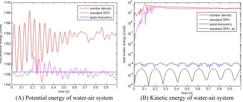
The stability of the interface is quantified by considering the potential and kinetic energy of the water-air system. The results in Figure 4 show that the potential energy remains practically constant in time when using the QB model, whereas it is fluctuating with standard SPH and with the number density approach. The kinetic energy with QB model is more than five orders lower (factor 10−5_{) than that with standard SPH and the number density approach. The result is the} closest to that of a single-phase simulation without interface, which is included as a reference. Even in this reference case, the kinetic energy is not zero because of errors in the particle approximation; however, it is small. It is thus demonstrated that with the QB model, a converged solution with stable interface is obtained.

(A) Unstable interface after t = 0.05 s (B) Unstable interface after t = 0.05 s

FIGURE 2 Stagnant flow in tank with periodic boundaries. A, Standard smoothed particle hydrodynamics without interface treatment;

B, Number density approach (Colagrossi et al10_{). Gravity acts vertically downwards, with the denser fluid beneath the less dense fluid. Static}

ghost particles at the bottom of the tank and the top is left open. The density ratio between the lighter fluid (blue circles) and water (red circles) is 1:1000 as indicated by the density color bar. The viscosity ratio is 10−5_:10−3_{, and the wave speed ratio is 15:60 [Colour figure can be}

viewed at wileyonlinelibrary.com]

(A) Stable interface at t = 0.5 s (B) Interface becomes slightly unstable after t = 1.0 s

FIGURE 3 Stagnant flow in tank with quasi-buoyancy model. The density ratio is 1:1000, viscosity ratio is 10−5_:10−3_{, and wave speed ratio}

is 15:60 [Colour figure can be viewed at wileyonlinelibrary.com]

(A) Potential energy of water-air system (B) Kinetic energy of water-air system

5.2

Rayleigh-Taylor instability

The second case is the Rayleigh-Taylor instability as studied by Cummins and Rudman,1 _{followed by Hu and Adams,}3 Colagrossi et al,10_{Grenier et al,}12_{and Monaghan.}14_{In this case, the denser fluid on top of a less dense fluid sinks under} gravity when a surface or interface perturbation is applied.

The density of the less dense fluid is 1000 kg/m3_{, whereas the density ratio is 1.8. The width of the fluid domain is 1} (0<x<1), and the height is 2 (0<y<2). The initial position of the perturbed interface is described by the function: y=1–0.15 sin (2πx). The Froude number is set toFr=1. The Reynolds number is set toRe=420. From these numbers, a characteristic fluid velocity is obtained and the dynamic viscosity, keeping the kinematic viscosity the same for the 2 fluids. Surface tension is neglected, which is acceptable with a relatively large radius of curvature of the order of 0.1 m.

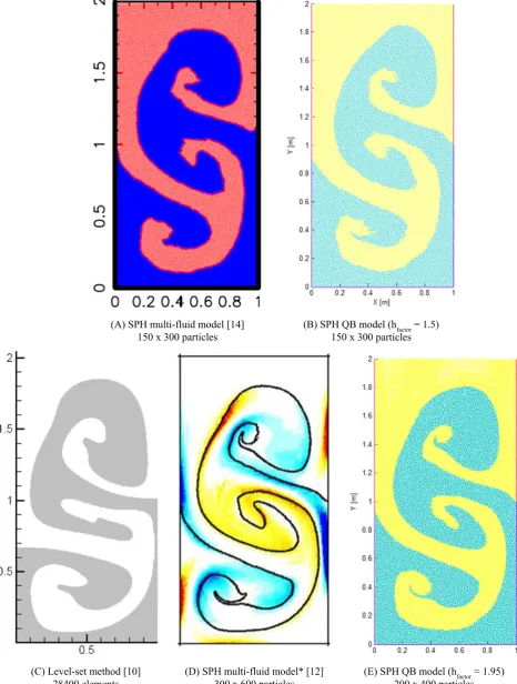
Simulations are made on an initially uniform grid at very low, low, medium, and high resolution: 50×100=5000 particles, 100×200=20000, 150×300=45000, and 200×400=80000 particles, respectively. In Figure 5, the results of 2 simulations with the QB model are presented with 3 results from the literature. The SPH QB model (Figure 5B,E) is compared with SPH multi-fluid models from Monaghan and Rafiee14_{(Figure 5A) and Grenier et al}12_{(Figure 5D) and} with a level-set method (Colagrossi et al10_{) (Figure 5C). From these results, it can be concluded that the development of} the mushroom-like shapes agree reasonably well. The 2 SPH results with medium resolution (150×300 particles) are similar but show some differences with the level-set solution, in particular, the shape of the fingers after the roll-up. The 2 SPH simulations with high resolutions show a better agreement with the level-set solution. In these cases, the interface is smoother, while the length and thickness of the fingers, including the details at the finger tips, are simulated better. The agreement between the SPH simulation from the work of Grenier et al12_{(resolution 300×600 particles) and SPH} simulation with QB model (resolution 200×400 particles) is excellent.

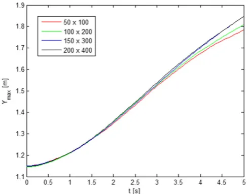
In Figure 6, the maximum height of the low-density fluid (yellow) is plotted in time for the aforementioned four reso-lutions. The results obtained with the medium and high resolutions are practically the same, indicating that convergence has been reached. From the results, it is concluded that the fluid accelerations are relatively small (a< <g) and, in this case, could be left out of the QB correction.

5.3

Rising bubble

The third case is a rising bubble as studied by Colagrossi and Landrini6_{and Sussman et al.}23_{In this case, the rise of an} air bubble in water is simulated and compared with a level-set solution from literature. The initial radius of the bubble isR=0.025 m. The density of the air and water phases are 1 kg/m3_{and 1000 kg/m}3_{, and the viscosities are 1.78×10}−5 Ns/m2_{and 1.137×10}−3_Ns/m2_{, respectively. The Bond number Bd=200, corresponding to a surface tension coefficient} 𝜎=0.1225 N/m. All values are chosen the same as in the work of Sussman et al,23_{whereas the work of Colagrossi and} Landrini6 _{adapts an artificial viscosity. The width and height of the fluid domain are 6Rand 10R, respectively, whereas} the gravitational accelerationg=9.8 m/s2_.

The choice of the artificial wave speeds is based on 2 conditions. The first condition is a sufficiently small Mach number M<0.1, which is commonly used in WCSPH. This condition is satisfied by choosing c> 10vmax, wherevmax is the maximum velocity in the fluid domain. The second condition is a prescribed wave speed ratiocair:cwater=1:4. This ratio of wave speeds is physically correct and close to the ratio of real wave speeds (cair=343 m/s andcwater=1282 m/s at 20◦C). On the basis of these 2 conditions, the artificial wave speeds are chosen ascair=5 m/s andcwater=20 m/s.

Note that in work of Colagrossi and Landrini,6_{the choice of the wave speeds is based on a different third condition: The} compressibility, represented by the term (𝜌0c02/𝛾) in the equation of state in Equation (13), is chosen the same for both fluids. With a density ratio of 1:1000,𝛾air=1.4 and𝛾water=7, their wave speeds arecair=198 m/s andcwater=14 m/s. This condition is usually applied in the particle number density approach (see, eg, the works of Colagrossi et al10_{and Grenier} et al12_{) so that the (change of) particle volume (under compression or expansion) is the same for both fluids, (Vj=Vi).} In this approach, the density of the fluid across the interface is taken the same (𝜌j=𝜌i) so that the particle mass can conveniently be replaced (𝜌jVj=𝜌iVi). It is implicitly assumed that the pressures are the same (pj=pi), ignoring the (change of) pressure gradients. The third condition leads to physically incorrect wave speed ratios. In the SPH modeling of heat transfer, physically correct wave speed ratios are essential although artificial wave speeds are allowed.

(A) SPH multi-fluid model [14] 150 x 300 particles

(C) Level-set method [10] 28400 elements

(D) SPH multi-fluid model* [12] 300 x 600 particles

(E) SPH QB model (h_factor = 1.95) 200 x 400 particles (B) SPH QB model (h_factor = 1.5)

150 x 300 particles

FIGURE 5 Rayleigh-Taylor instability aftert=5 s. Comparison of quasi-buoyancy (QB) model with multi-fluid models from the literature. Top row: smoothed particle hydrodynamics (SPH) simulations with medium resolution. Bottom row: level-set and SPH simulations with

FIGURE 6 Rayleigh-Taylor instability. Convergence study for the time evolution of the measured maximum height of the lighter fluid. The red, green, blue, and black lines indicate the very low, low, medium, and high resolution, respectively [Colour figure can be viewed at wileyonlinelibrary.com]

The results of SPH simulations with QB model and without (standard SPH) are presented in Figure 7 and compared with the bubble contour obtained with a level-set method from Sussman et al.23_{At early stages (dimensionless timet} (g/R)1/2_{≤3.6), the results are very similar. However, later on, the bubble rises too quickly with standard SPH, which may} be attributed to the particle instability at the interface (see Section 2). As discussed in Section 2.2, an air particle near the interface tends to move upwards because of a higher (hydrostatic) pressure of a water particle beneath it (Figure 1). In the same way, it also tends to move upwards because of the lower (hydrostatic) pressure of a water particle above it. In the simulation with the QB model, the rise of the bubble is stabilized, and its rise and deformation is in an overall agreement with the level-set solution. However, there are some differences: (1) The thickness of the horseshoe at the line of symmetry is larger than in the level-set solution, and (2) during the roll-up of the horseshoe, one secondary bubble is formed at each tip, where the level-set solution shows the temporary existence of 2 smaller bubbles. Both observations (1) and (2) are also seen in the SPH results presented in the work of Colagrossi and Landrini.6_{With standard SPH, instead of} the formation of smaller bubbles, a dispersion of particles is seen along the path of the smaller bubbles. This dispersion may again be attributed to the particle instability at the interface. With the QB model the dispersion is hardly present because of the fact that it deals with true buoyancy (Section 3.3).

In Figure 8, the results of a convergence study are presented on the basis of simulations with 3 resolutions: Np =150×250= 37 500 particles, 4Np = 300×500=150 000 particles, and 16Np =600×1000=600 000 particles. With increasing resolution, the bubble contour converges to the contour of the level-set solution (red dots). In the high-resolution case, the bubble position is very similar as well as the bubble shape, indicating in a qualitative way that convergence is reached.

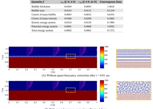
The convergence is quantified according to the method described in the work of Colagrossi and Landrini.6_{The results} are given in Table 1, where the relative changeεbetween 2 simulations with subsequent resolutions (N, 4N, and 4N, 16N particles) is given for some local and global quantitiesf. The local quantities are the thickness (at center linex=0), area, center of mass, and center of the mass velocity of the air bubble. The global quantities are the potential, kinetic, and total energy of the entire water-air system. The relative changes between the medium and high resolution (column 3) are within 1.3% except for the center of mass velocity, indicating that a reasonable level of convergence is reached. The convergence rate, defined as log (𝜀32/𝜀21) /log(2), is given in the right column.

5.4

Air flow along a water surface

QS-model | standard SPH QS-model | standard SPH QS-model | standard SPH

FIGURE 7 Rising bubble. Smoothed particle hydrodynamics simulation with quasi-buoyancy model (left half) versus standard smoothed

particle hydrodynamics (right half), compared with a level-set solution23_{(red dots) [Colour figure can be viewed at wileyonlinelibrary.com]}

A special type of particles is used to form a top wall, where the density and pressure are evaluated as usual, while no motion is allowed. The suction effect of these particles prevents the formation of cavities near the wall because of under pressure. We have applied the concept successfully to pipe walls. It is similar to the quasi-fluid boundary particles, introduced by Valizadeh et al.24

(A) 150 x 250 particles (B) 300 x 500 particles (C) 600 x 1000 particles

FIGURE 8 Rising bubble. Convergence test, smoothed particle hydrodynamics results with quasi-buoyancy model. A, low resolution; B, medium resolution; C, high resolution [Colour figure can be viewed at wileyonlinelibrary.com]

TABLE 1 Rising bubble. Convergence test with relative changes𝜀of quantityf

between resolutionsNand 4N(column 2) and 4Nand 16N(column 3) and

convergence rate (column 4) at dimensionless instant of timet(g/R)1/2_=4.0

Quantityf 𝜀21(f,N, 4N) 𝜀32(f, 4N, 16N) Convergence Rate

Bubble thickness 0.0369 0.0093 1.9810

Bubble area 0.0143 0.0131 0.1234

Center of mass bubble 0.0083 0.0052 0.6593

Center of mass velocity 0.0360 0.0290 0.3083

Kinetic energy system 0.0218 0.0129 0.7489

Potential energy system 0.0001 0.0008 3.0382

Total energy system 0.0002 0.0003 0.7372

(A) Without quasi-buoyancy correction after t = 0.01 sec

(B) With quasi-buoyancy correction after t = 1.0 sec

FIGURE 9 Air flow along water surface. Results of simulations with and without quasi-buoyancy model. The density ratio is 100, the

A typical result of a simulation is shown in Figure 9. The air velocity is 5 m/s at the top, while the artificial wave speeds arec=15 m/s andc=60 m/s for air and water. Without QB correction, the interface becomes unstable soon after the start of a simulation. With correction, the interface remains however stable in time. No particle clustering or layering occurs. The results demonstrate the capability of the QB model to deal with high density ratios at realistic wave speed ratios and significant fluid velocities.

FIGURE 10 Internal gravity waves. Initial particle and velocity distribution,𝜌hand𝜌lrepresent the high- and low-density fluid, respectively [Colour figure can be viewed at wileyonlinelibrary.com]

t = 0.0 s

t = 1.0 s

t = 2.0 s

t = 3.0 s

t = 4.0 s

5.5

Internal gravity waves

The fifth case is about the propagation of internal gravity waves, a case described by Dean and Dalrymple.25_{The fluid} domains are 0≤x≤10.0 and−0.4≤y≤2.0, with static ghost particles placed at the sides and bottom of the domain. A hexagonal particle distribution with an interparticle distance of d=0.02 is used as the initial condition. The total number of particles, including fluid and ghost particles, isNp=40000.

SPH particles with equal initial volume are also utilised to setup the initial particle distribution of the multi-fluid simu-lation. The initial perturbation in the work of Valizadeh et al24_{is employed to prescribe the interface and velocity profiles} for both single- and multi-fluid simulations. The initial conditions are setup such that the unperturbated interface is located aty=0. The depth of the heavy fluid (subscripth) is 0.3 m, and the initial wave height is 0.21 m. The initial inter-face and velocity profiles are given in Figure 10. Without loss of generality, the fluid properties such as speed of sound (ch=20 m/s,cl=15 m/s), polytropic exponents (𝛾h=7,𝛾l=1.4), and the base density of the heavy fluid𝜌h=1000 kg/m3 are deliberately kept constant in all cases. The kinematic viscosity is also constant, and𝜈=0.001 m2_{/s for both fluids. The} internal gravity waves for 3 density ratios𝜌h/𝜌l=2, 5, and 100 are simulated untilt=4.0 s.

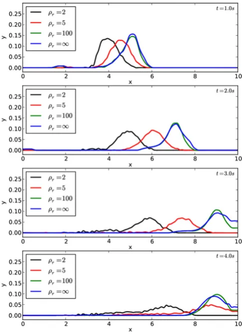
In the single-fluid case, the perturbation leads to free-surface waves, whereas for the multi-fluid case, the perturbation generates internal gravity waves between the 2 fluids. The growth of the internal wave excites the interface between the 2 fluids and eventually generates free-surface waves at the top of the light fluid. The results of a simulation performed at a density ratio of 100 is given in Figure 11. The initial perturbed wave propagates in the positive x-direction and generates free-surface waves, which lag the internal wave. The results of the multi-fluid simulations and single-fluid simulation are plotted together in Figure 12. As expected, the difference decreases with increasing density ratio and converges to the free-surface flow solution (ie,𝜌h/𝜌l→∞). In the latter case, the wave propagationc=2.03 m/s (ie, between 0<t<3 s), which agrees reasonably well with the theoretical free surface wave propagationc=√g h=1.98 m/s, whereg=9.8 m/s2 andh=0.4 m (including the bottom particle layer).

FIGURE 12 Internal gravity waves. Results of 3 multi-fluid simulations and 1 single-fluid simulation. Interface profiles at density ratios 2,

5, and 100 (multi-fluid) and free-surface profile at density ratio of∞(single fluid) at various instants of time [Colour figure can be viewed at

6

S U M M A RY A N D CO N C LU S I O N S

The interface between 2 fluids is characterized by a discontinuity in the pressure gradient. This results in a force imbalance for SPH particles near the interface, which is attributed to the particle approximation. To stabilize the interface, a new concept is introduced and explored to deal with the change of pressure gradient because of the discontinuity of the density. A distinction is made between the hydrostatic and nonhydrostatic pressure gradient because of the gravitational and fluid acceleration, respectively.

The concept is based on a density correction. In the first instance, a quasi-buoyancy force is evaluated from a mixture density around the interface. This additional force is used to balance the (erroneous) SPH hydrostatic pressure force. In the second instance, the pressure gradient is related to the gravitationalandfluid accelerations via the Euler equations. The pressure force is derived formally from the kernel instead of the kernel gradient. The resulting additional force is essentially the same as the QB force, but now, the fluid acceleration is included in the density correction, which makes the concept also applicable to nonhydrostatic flows.

The concept is introduced as the “quasi-buoyancy” model. The interface stabilization method is based on physics. No parameters or coefficients are involved. It may be applied to other formulations of the SPH momentum equation than used in this paper. It may be applied to confined flows and free-surface flows.

The QB model is explored in 5 case studies.

• The stagnant flow case demonstrates the particle instability, revealed by particle clustering and layering at high den-sity ratios, if no interface stabilization is applied. The QB correction keeps the interface stable. The kinetic energy of the water-air system remains low and close to that in a single-phase simulation, while the potential energy remains constant. The concept is compared with 3 multi-fluid models in literature. It is demonstrated that it better performs at high density ratios (here, 1000) and realistic wave speed ratios (here, 4).

• The Rayleigh-Taylor instability case shows a reasonable agreement with a level-set method and a good agreement with other SPH multi-fluid models from the literature.

• The rising bubble case shows an overall agreement with a level-set method from the literature, although the temporary smallest bubbles are not seen (like in other SPH multi-fluid models). Real viscosities are used like in the level-set method.

• It is demonstrated that an air flow along a water surface can be simulated up to high density ratios, together with real viscosities, realistic wave speed ratios, and relatively high fluid velocities.

• The propagation of internal gravity waves can be simulated up to high density ratios of 100, together with more realistic wave speed ratios than found in the literature.

The cases demonstrate that the QB model allows for high density ratios and real (low) viscosities, while no particle clustering or layering occurs at the interface. No (other) stabilization techniques such as artificial viscosity, Shepard filter, XSPH, delta SPH, and/or particle shifting methods are used here.

The QB model allows for the modeling of multi-fluids with realistic wave speed ratios as long as the fluid velocities are not very high, where other WCSPH multi-fluids models rely on (physically unrealistic) artificial ratios. Although the SPH wave speeds may be artificial in many cases, correct and realistic wave speed ratios are essential in the modeling of heat transfer between 2 fluids.

To summarize, a QB model is introduced that stabilizes the interface between 2 fluids by effectively introducing a buoyancy force that counteracts the force because of an incorrectly calculated pressure gradient near to any interface. It is demonstrated that this correction works well in 5 case studies and provides an improvement on WCSPH multi-fluid models currently available in the literature aimed at alleviating this problem. The multi-fluid model is easy to implement, and on the basis of the particle approximation, it fits well within the WCSPH method.

AC K N OW L E D G E M E N T S

The work was funded by Rolls-Royce and the European Union within the research project ELUBSYS (Engine Lubrication System Technologies) under grant ACP8-GA-2009-233651. This financial support is gratefully acknowledged.

O RC I D

R E F E R E N C E S

1. Cummins SJ, Rudman M. An SPH projection method.J Comput Phys. 1999;152(2):584-607.

2. Hu XY, Adams NA. An incompressible multi-phase SPH method.J Comput Phys. 2007;227(1):264-278.

3. Hu XY, Adams NA. A constant-density approach for incompressible multi-phase SPH.J Comput Phys. 2009;228(6):2082-2091.

4. Xu R, Moulinec C, Stansby P, Rogers BD, Laurence D. Simulation of vortex spindown and Taylor-Green vortices with incompressible SPH method. Paper presented at: 3rd ERCOFTAC SPHERIC Workshop on SPH Applications; 2008; Lausanne, Switzerland.

5. Ritchie BW, Thomas PA. Multiphase smoothed-particle hydrodynamics.Mon Not R Astron Soc. 2001;323(3):743-756.

6. Colagrossi A, Landrini M. Numerical simulation of interfacial flows by smoothed particle hydrodynamics. J Comput Phys.

2003;191(2):448-475.

7. Flebbe O, Münzel S, Herold H, Riffert H, Ruder H. Smoothed particle hydrodynamics: physical viscosity and the simulation of accretion

disks.Astrophys J. 1994;431(2):754-760.

8. Ott F, Schnetter. A modified SPH approach for fluids with large density differences. 2003. http://arxiv.org/abs/physics/0303112

9. Hu XY, Adams NA. A multi-phase SPH method for macroscopic and mesoscopic flows.J Comput Phys. 2006;213(2):844-861.

10. Colagrossi A, Antuono M, Grenier N, Le Touzé D, Molteni D. Simulation of interfacial and free-surface flows using a new SPH formulation. Paper presented at: 3rd ERCOFTAC SPHERIC Workshop on SPH Applications; 2008; Lausanne, Switzerland.

11. Adami S, Hu XY, Adams NA. A new surface-tension formulation for multi-phase SPH using a reproducing divergence approximation.

J Comput Phys. 2010;229(13):5011-5021.

12. Grenier N, Antuono M, Colagrossi A, Le Touze D, Alessandrini B. An Hamiltonian interface SPH formulation for multi-fluid and free

surface flows.J Comput Phys. 2009;228(2):8380-8393.

13. Monaghan JJ. SPH without tensile instability.J Comput Phys. 2000;159(2):290-311.

14. Monaghan JJ, Rafiee A. A simple SPH algorithm for multi-fluid flow with high density ratios.Int J Num Methods Fluids. 2013;71(5):537-561.

15. Khayyer A, Gotoh H, Ikari H, Tsuruta N. A novel error-minimizing scheme to enhance the performance of compressible-incompressible multiphase projection-based particle methods. Paper presented at: 8th International SPHERIC Workshop; 2013; Trondheim, Norway. 16. Khayyer A, Gotoh H. Enhancement of performance of stability of MPS mesh-free particle method for multiphase flows characterized by

high density ratios.J Comput Phys. 2013;242:211-233.

17. Lind SJ, Stansby PK, Rogers BD. Incompressible-compressible flows with a transient discontinuous interface using smoothed particle

hydrodynamics (SPH).J Comput Phys. 2016;309:129-147.

18. Lind SJ, Stansby PK, Rogers BD, Lloyd PM. Numerical predictions of water-air wave slam using incompressible-compressible smoothed

particle hydrodynamics.J Appl Ocean Res. 2015;49:57-71.

19. Murnaghan FD. Finite deformation of an elastic solid.Am J Math. 1937;59(2):235-260.

20. Price DJ. Magnetic Fields in Astrophysics [PhD Thesis]. Cambridge, UK: University of Cambridge; 2004.

21. Wendland H. Piecewise polynomial, positive definite and compactly supported radial functions of minimal degree.Adv Comput Math.

1995;4(4):389-396.

22. Hou Q, Kruisbrink ACH, Pearce FR, Tijsseling AS, Yue T. Smoothed particle hydrodynamics simulations of flow separation at bends.

J Comput Fluids. 2014;90:138-146.

23. Sussman M, Smereka P, Osher S. A level set approach for computing solutions to incompressible two-phase flow.J Comput Phys.

1994;114(1):146-159.

24. Valizadeh A, Shafieefar M, Monaghan JJ, Salehi Neyshaboori SAA. Modeling two-phase flows using SPH method. J Appl Sci.

2008;8(21):3817-3826.

25. Dean RG, Dalrymple RA.Water wave mechanics for engineers and scientists. Singapore: World Scientific Co; 1991. Advanced Series on

Ocean Engineering; vol 2.

A P P E N D I XA

Q B C o r re c t i o n D e r i ve d f ro m Eu l e r E q u a t i o n s

In this section, the pressure force on a particle is evaluated from the Euler equations to provide a pressure gradient correc-tion near the interface. Consider a single inviscid fluid in a gravitacorrec-tional field. The pressure force on particlei, according to the Euler equations, is related to the fluid acceleration by

⃗ F_𝑝,i=𝜌i

(

⃗

ai−⃗g)Vi, (A.1)

whereaiis the acceleration of particlei. Applying the particle approximation in Equation (1) to the product of density and acceleration in Equation (A.1) results in

⟨

𝜌i

(

⃗

ai−⃗g)⟩=∑

𝑗

𝜌𝑗(a⃗𝑗−⃗g)V𝑗W𝑖𝑗. (A.2)

Thus, the pressure force may be estimated from

⃗ F_𝑝,i=

∑

𝑗

𝜌𝑗(⃗a𝑗−⃗g)ViV𝑗W𝑖𝑗. (A.3)

Now, the step from single fluid to multi-fluid is made. Hereby, a distinction is made between neighbor particlesj∈fluid

𝛼andj∈fluid𝛽

⃗ F_𝑝,i=

∑

𝑗∈𝛼

𝜌𝑗,𝛼(a⃗𝑗−⃗g)ViV𝑗W𝑖𝑗+

∑

𝑗∈𝛽

𝜌𝑗,𝛽(⃗a𝑗−⃗g)ViV𝑗W𝑖𝑗. (A.4)

It is obvious that because of the density difference, the contribution of the second term to the pressure force is rather different from that in a single-fluid flow. Now, suppose that all particlesj∈fluid𝛼. For this purpose, the density of particles j∈fluid𝛽is replaced by an (unknown) virtual density (𝜌j*) as if they belong to fluid𝛼. The above pressure force may now be written as

⃗ F_𝑝,i=

∑

𝑗∈𝛼

𝜌𝑗,𝛼(a⃗𝑗−⃗g)ViV𝑗W𝑖𝑗+

∑ 𝑗∈𝛽 𝜌∗ 𝑗,𝛽 ( ⃗

a_𝑗−⃗g)ViV_𝑗W_𝑖𝑗 +∑

𝑗∈𝛽

(

𝜌𝑗,𝛽−𝜌∗𝑗,𝛽

) (

⃗

a_𝑗−⃗g)ViV_𝑗W_𝑖𝑗. (A.5)

The first and second terms on the right-hand side of this equation describe the pressure force in a single fluid, ie, as if all neighbour particlesj∈fluid𝛼. The third term describes the contribution of the other fluid𝛽to the pressure force, ie, some of the neighbor particlesj∈fluid𝛽. It is this term that quantifies the force imbalance for particles near the interface. The virtual density (𝜌j*) in Equation (A.5) is not known exactly. For a first approximation, it may be assumed that the virtual pressure of neighbor particlesj∈fluid𝛽is equal to that of particlei(pj*≈pi). This may be seen as a Neumann boundary condition across the interface. If these particlesjare treated as if they belong to fluid𝛼, then the virtual density is equal to the real density of particlei(𝜌j*≈𝜌i).

The third term in the previous equation may now be used as pressure force correction, simply by taking the opposite sign. This yields

ΔF⃗_𝑝,i=

∑

𝑗∈𝛽

(

𝜌𝑗−𝜌i

) (

⃗

g−a⃗_𝑗)ViV_𝑗W_𝑖𝑗. (A.6)

This result is essentially the same as that in Equation (7), and it is also based on a density correction. Here, it is derived in a more formal way. With the inclusion of the fluid acceleration, the concept is more generally applicable.

A P P E N D I XB

C o m p a r i s o n w i t h M u l t i- fl u i d M o d e l f ro m H u a n d Ad a m s2

In this appendix, the interface treatment of Hu and Adams2 _{is applied to a multi-fluid case with hydrostatic pressure} distribution and a high density ratio.

Hu and Adams,2_{followed by Adami et al,}11_{stabilized the interface with a density weighted interparticle pressure defined} as

𝑝𝑖𝑗= 𝜌i𝑝_𝜌𝑗+𝜌𝑗𝑝i i+𝜌𝑗

The above pressure is used in the particle number density form of the momentum equation to ensure a continuous pressure gradient in a discontinuous density field. As such, it may be considered as a pressure gradient correction.

To allow for a comparison, we consider the hydrostatic pressure distribution around an interface as shown in Figure 1, which may be written as

𝑝=𝑝_𝛼𝛽+𝜌g (h_𝛼𝛽−z), (B.2)

wherep_𝛼𝛽is the pressure at the interface levelh_𝛼𝛽. Now, consider a particlei∈fluid𝛼and particlej∈fluid𝛽. Substitution of Equation (B.2) in Equation (B.1) gives, after some manipulation,

𝑝𝑖𝑗 =𝑝𝛼𝛽+

[

2𝜌_𝑗

𝜌i+𝜌𝑗

]

𝜌ig

(

h_𝛼𝛽− zi+z𝑗

2

)

. (B.3)

To ensure a stable interface, the average pressure of the multi-fluid particle pair should be the same as that in a single fluid (𝜌j≈𝜌i), which, according to Equation (B.2), results in

𝑝𝑖𝑗 = 𝑝i+𝑝𝑗

2 =𝑝𝛼𝛽+𝜌ig

(

h_𝛼𝛽−zi+z𝑗

2

)

. (B.4)

(A) Stable interface at t = 0.5 s (B) Interface becomes unstable after t = 1.0 s

FIGURE B1 Stagnant flow in tank. Density ratio is 1:1000. Wave speed ratio is 15:30 [Colour figure can be viewed at wileyonlinelibrary.com]

(A) Interface becomes unstable after t = 0.5 s (B) Unstable interface at t = 1.0 s

It can be easily seen that the 2 results for an averaged pressure are the same if the interface lies at the midpoint between the particlesiandj. This is the assumption made in the work of Hu and Adams.2_{In general, this is not true. The hydrostatic} pressure gradient felt by particleimust bedp/dz= −𝜌ig. The term between square brackets in Equation (B.3) describes the error made with the interparticle pressure.

The multi-fluid model is applied to the case study “stagnant flow in tank” (Section 5.1). The results are shown in the Figures B1 and B2. For a wave speed ratio of 15:30, the model behaves reasonable well. However, for a more realistic wave speed ratio of 15:60, the model fails soon after the start of the simulation.

A P P E N D I XC

C o m p a r i s o n w i t h M u l t i- fl u i d M o d e l f ro m M o n a g h a n1 4

In this appendix, the interface treatment of Monaghan and Rafiee14 _{is applied to a multi-fluid case with hydrostatic} pressure distribution and a high density ratio.

Monaghan and Rafiee14_{stabilized the interface with the following repulsive force:}

ΔFr_,i= −

∑

𝑗

mim_𝑗0.08||||

| (_𝜌

0,i−𝜌0, 𝑗 𝜌0,i+𝜌0, 𝑗

) _𝑝

i+𝑝𝑗 𝜌i𝜌𝑗

|| ||

|∇iW𝑖𝑗. (C.1)

The force is based on a pressure gradient similar to that seen in Equation (15) and, as such, may be considered as a pressure gradient correction. The concept is based on an artificial back ground pressure.13

Substitution of the hydrostatic pressure distribution from Equation (B.2) in Equation (C.1) gives

ΔF_r,i= −∑

𝑗

ViV𝑗0.08||||

| (

𝜌0,i− 𝜌0, 𝑗) (_𝜌 𝜌0, 𝑗 0,i+𝜌0, 𝑗

)

g(h_𝛼𝛽−z_𝑗)||||

|∇iW𝑖𝑗. (C.2)

Note that the constant terms (ie,piandp_𝛼𝛽) are left out of the equation since they vanish under the kernel gradient summation.

The difference between the hydrostatic pressure in a multi-fluid (i∈𝛼,j∈𝛽) and single fluid (i∈𝛼,j∈𝛼) follows from Equation (B.2) (see Figure 1)

𝑝𝑗,𝛽−𝑝𝑗,𝛼=(𝜌0,𝑗−𝜌0,i)g(h𝛼𝛽−z_𝑗). (C.3)

(A) Unstable interface at t = 0.05 s (B) Unstable interface at t = 0.5 s

This pressure difference is the excess pressure that tends to move particleiupwards (Section 2.2). Adding this excess pressure as an extra term in the equation of motion in Equation (15) and taking the opposite sign would give a pressure force correction

ΔF_𝑝,i= −∑

𝑗 ViV𝑗

(

𝜌0,i−𝜌0,𝑗)g(h𝛼𝛽−z𝑗)∇iW𝑖𝑗. (C.4)

Comparing the aforementioned 2 approaches suggests that the repulsive force in Equation (C.2) is not consistent with the correction in Equation (C.4), which is needed for a hydrostatic pressure distribution. Moreover, the coefficient 0.08 seems to be case specific. For high density ratios, the repulsive force seems too small, which is confirmed by the results below.