Fuzzy Logic based Power Factor Control of
Synchronous Machine
Ahmed Nasser B. Alsammak
,
PhD
Assistance Professor
University of Mosul
College of Engineering
Electrical Engineering Department
Mosul-Iraq
ABSTRACT
In this paper, a fuzzy logic technique is used to control the power factor (PF) that compensate the reactive power of the load by controlling the excitation system of synchronous machine. This fuzzy logic controller can give a fast response compensation to meet the required load reactive power and hence keeping the load bus at constant set point PF value. The V curve of PF is treated in a way to get the flexibility and the limitation the over or under values, as well as time delay could therefore be eliminated with such a control configuration. The results show that fuzzy based power factor controller using synchronous machine is reliable, sensitive, faster and more efficient compare with the other methods such as capacitor groups.
Matlab-Simulink program was adopted for the architecture and learning procedure of fuzzy system depending of construct an input-output mapping based on both knowledge and stipulated input-output data pairs. A model of the synchronous machine was also presented in this paper. The variable DC voltage based excitation field current controller was built based on fuzzy logic controller to generate the firing angle of six-pulse rectifier circuit.
Keywords
Fuzzy logic controller, Power factor controller, Synchronous machine model, and Reactive power compensation.
List of Symbols:
SM = Synchronous machine.
va, vb and vc = Thee phase terminal voltages (Volt). ia, ib and ic = Thee phase terminal current (Ampere). = Firing angle (degree).
Vf= DC field voltage (volt). If= DC field current (amper). Rf= Resistance of field circuit (ohm). Lff= Self of rotor inductance (henry).
La, Lb and Lc= Stator self-inductance (static)/ phase (henry). Lab, Lbc and Lca= Mutual inductance between stator Phases (henry).
Laf, Lbf and Lcf= mutual inductances between stator phases and rotor (henry).
Ls= Part of phase inductance harmonic because of salience (henry).
a, b and c= Instantaneous linkage flux for stator phases (Wb).
f = Instantaneous linkage flux for rotor (Wb). [V]= Voltage matrix (volt).
[R]= Resistance matrix (ohm). [i]= Current matrix (amper). []=Linkage flux matrix (Wb). [L]= Inductance matrix (henry). Te= Electrical torque (N.m). TL= Mechanical torque (N.m). s= Synchronous speed (rpm). r= Rotor speed (rpm).
= Displacement angle for rotor refers to stator phase (a) (rad).
Vf =DC field voltage (volt).
PL&QL = Real and reactive power load demand respectively (watt, var).
Pm&Qm = Real and reactive power of the Synchronous machine respectively (watt, var).
Pt&Qt = Total real and reactive power for the Synchronous machine and load demand respectively (watt, var).
1.
INTRODUCTION
correction without step changes. In industry, most of the reactive power compensation systems have been achieved by using constant capacitor groups, which are controlled by contactors and timers [6]. In this case, the penalties such as time delay, over compensation or lower compensation are always possible because of the step changes of capacitor groups. In addition, capacitors are often less flexible and less economical. On the other hand, synchronous machine (SM) can operate at unity, lagging or leading PF condition, so that the SM can be provide network by the reactive power demand [7].
Presently for the smooth and fast reactive power compensation, SM will be widely used for the reactive power compensation due to low cost of the compact system, SM and controller, as compared with power electronics with capacitor grope, Flexible AC Transmission System (FACTS) [8]. In addition, SM minimal harmonics content and, therefore, require no special filtering [9].
2.
DETERMINATION OF CAPACITOR
POWER
A system with the installed active power P is to be compensated from a power factor cos φ1 to a power factor cos φ2. The capacitor power necessary for this compensation is calculated as follows: Qc = P · (tan φ1 – tan φ2)
[image:2.595.318.528.87.635.2]Compensation reduces the transmitted apparent power S, as shown in Figure 1. Ohmic transmission losses decrease by the square of the currents.
Fig. 1: Power diagram for a non-compensated (1) and a compensated (2) installation.
3.
VOLTAGE STABILITY AND POWER
FACTOR
In a practical calculation for a complex power system, the fall in system voltage as the load rises must be assumed to operate the on load tap changer (OLTC). When these reach their limits, and VAR Compensator VC equipment reach to limit also, the system voltage will continue to fall as the load rises. The single line diagram of a 2-Bus system is shown in Figure 2. It can be seen form result in Figure 3 that the variation of voltage stability margin is wide for lagging PF values up to unity PF while this margin is narrow for leading PF. Increasing voltage levels by OLTC action can decrease the margin of voltage stability due to the effect of increasing the inductively reactive power in to the load side, in case the VC equipment reaches its limit in providing reactive power [9, 10].
[image:2.595.332.526.218.393.2]The critical voltage can be kept constant with the variation of both PF and power. Figure 4 shows the variation of reactive power with voltage for different constant values of real power [7, 11].
[image:2.595.55.291.387.548.2]Fig.2: The single line diagram of a 2-Bus system.
Fig.3: Normalized p-v curves for two bus system,
Where Vr
Vs
v
, 2
PX s V s
p
.
Fig.4: Normalized v-q curves for two bus system, where
Vr Vs
v
, 2
QX s V s
q
.
4.
MODELING OF SYNCHRONOUS
MACHINE
The direct 3-phase model of the SM can be represented by the following equations [12]:
V
R
i
p
L
i
…(1) …(2.1)
V
R
i
p
…(2)
ta b c f
i
i
i
i
i
…(3) …(2.3)
R diag
Ra Rb Rc Rf
…(4)
tf
a b c
V
v
v
v
V
…(5)
ta b c f
p
p
p
p
p
…(6) Since, the relationship between leakage flux and current is:
L
i
…(7)where [L] matrix given in Table 1.
Differentiating two sides of equation (7) gives:
i
p
d
L
d
i
p
L
p
…(8) where matrix
d L dis given in Table 1. Rearranging equation (8) would result in:
i
p
d
L
d
i
R
V
L
i
p
1.
…(9) The total electrical developed torque would thus be [12]:
0.5
.
e
d L
T
i
i
d
…(10) dt d J dt d KD K TTe m r
…(11) All equations from (1) to (11) were modeled and simulated using MATLAB-Simulink. Figure 5 shows the overall suggestion system and Figure 6 shows the Matlab model.
5.
FUZZY LOGIC CONTROLLER
Fuzzy control is one of the most well-known fuzzy logic applications. In 1974, E. H. Mamdani was the first to demonstrate the application of fuzzy logic in control field [13]. A major breakthrough of fuzzy control came in the beginning of 1980's, where a controller development for a cement kiln was the first real application of fuzzy control. Within the next year, several successful applications were presented, where many of them had been exposed during the IFSA (International Fuzzy Systems Association) meeting in Tokyo 1987 [14, 15].
The objective is to design a FLC capable of keeping the plant PF at or above the desired threshold value by compensating load reactive power. The FLC will use both of the PF and error signal (e) of the SM as inputs to obtain the FLC output used to drive six-pulse full wave thyristorized rectifier circuit which can thus control the excitation field voltage. The SM would thus produce kVAR which will achieve the load reactive power at the desired SM PF.
The proposed FIS can construct an input-output mapping based on both human knowledge (in the form of fuzzy if-then rules) and stipulated input-output data pairs, for SM at no load, as shown in Figure 7-a, where the inverse V-curve has been treated in a way that all lagging PF less than unity PF are taken as its values, while all leading PF less than leading unity
were processed in such a way that the zero leading PF value is considered to be equal to 2, the whole leading PF range would thus be in the range of :
1
PFm
2
Leading
.
The designed FIS has two fuzzy variables (PF and error) and seven linguistic variables for each, PF from very Lag (VLa) to very Lead (VLe) and Error from negative big (NB) to positive big (PB). The FLC attributes and all details are summarized as follows and shown in the in Figure 7-b.
Name: 'PF controller'; type: 'sugeno'. AndMethod: 'prod'; orMethod: 'max'. DefuzzMethod: 'wtaver'; impMethod: 'prod'. AggMethod: 'sum'; input: [1x2 struct]. Output: [1x1 struct]; rule: [1x49 struct].
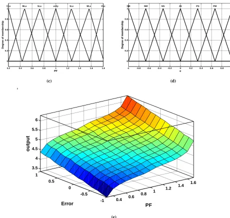
The membership functions of the input fuzzy variable are shown in Figure 7-c and Figure 7-d. The control surface is defined with 49 rules, as shown in Figure 7-e. A flowchart of reactive power compensation using fuzzy algorithm had been shown in Figure 8.
6.
SIMULATION RESULTS
Reactive power compensation of power system based on VAR/PF controller of SM could be made after the complete determination of the power system weak buses with the aid of the analysis and modeling using Q-V sensitivity. A computer program gives the effect of reactive power compensation on weak bus and overall system, which would thus give the state of the system voltage stability.
Simulation results of the SM and IEEE 14-buses sample system, shown in Figure 9, is presented and analyzed in this paper. The weak buses of IEEE 14-bus sample system are determined as shown in Figure 10. Numerous graphs showing in Figure 11 the behavior of the system in various conditions have been included to illustrate the analysis with various values of control action.
7.
CONCLUSIONS
PF fuzzy Controller for reactive power compensation is investigated in a single machine connected to infinite bus system with load. A controller introduced depends on the dynamic behavior of SM analysis. This machine is used to control the total reactive power absorbed by the load. An intelligent controller FIS have been designed, and compared to output control signal used to drive six-pulse full wave thyristorized rectifier circuit which can thus control the excitation field voltage. The SM (working as motor) will produce the needed kVAR, for the desired PF to the weak bus. Design of FLC give higher performance that overcome output response overshoot in both of the over or under compensations. The main benefits of this designed system would thus exist in more flexibility, fast (about two cycles), more efficient, reliable and economical.
Bifurcation analysis and Q-V sensitivity methods have been used to calculate system weak buses which are characterized by showing higher participation factors to the smallest Eigen-values. These methods have been applied on IEEE 14-Bus
MATLAB, PSAT. The weak load bus has been chosen for the SM reactive power compensation that would hence in turn result in improving the overall system voltage stability.
Fig.5: Overall suggested main system.
Pm+jQm
Load
Infinite
Bus
Networ
k
Synchronous Motor
+
-3 phase Supply
FLC (sugeno)
V
e PF
Pt+jQt
P
L+jQ
Lim
Calculate: PF
t, PF
SM,
PF
L, Q
t, Q
m, Q
L, all
real powers.
Fig.6: The overall main system model in MATLAB-Simulink.
(a)
(b)
3
3.8 4.6
5.4 6.2
7
-1 -0.5 0 0.5 1 0 0.5 1 1.5 2
output Error (e)
PF
System PF anfis controller: 2 inputs, 1 outputs, 49 rules
PF (7)
Error (7)
f(u)
output (49)
PF anfis controller
(sugeno)
49 rules
PF Controller(Sugeno)
49 rules
va&ia
theta u(10)
six pulse rectifier circuit
f(u) infinity Bus-Bar
van vbn vcn
f8(u) f(u) f7(u)
f(u) f6(u)
f(u) f5(u)
f(u)
f4(u)
f(u) f3(u)
f(u) f2(u)
f(u) f1(u)
f(u)
dif/dt u(8) dic/dt1
u(6) dib/dt1
u(4) dia/at
u(2)
Wr
u(11)
Vf Torque
f(u)
Sum4 Pt+jQt
Pt Qt
Pm+jQm
Pm Qm
PQSM PFref
PF
Output Results
PQm
PQt
Mux3 Mux
Mux2 Mux
Mux1
Mechanical load
Torque theta (elec)
speed (rpm)
Load and SM PQ
in1
in2 PQ
LOAD
PL+jQL
Integr.1
1/s
Integ.4 1/s Integ.3
1/s
Integ.2
1/s
Demux
Demux Controller
PQ
PFalpha
Active & Reactive Power
V I PQ
ia
dia/dt
ib
dib/dt
ic
dic/dt
if
dif/dt
Wr (mec .)
(c) (d)
[image:6.595.69.531.77.513.2](e)
Fig. 7: Proposed FLC where: (a) FIS input-output training, (b) FLC input-output structure, (c) PF fuzzy membership function. (d) Error signal fuzzy membership function. (e) Proposed FLC surface.
0.2 0.4 0.6 0.8 1 1.2 1.4 1.6 1.8 0
0.2 0.4 0.6 0.8 1
PF
D
e
g
re
e
o
f
m
e
m
b
e
rs
h
ip
VLa MLa SLa unity SLe MLe VLe
-1 -0.8 -0.6 -0.4 -0.2 0 0.2 0.4 0.6 0.8 1 0
0.2 0.4 0.6 0.8 1
e
D
e
g
re
e
o
f
m
e
m
b
e
rs
h
ip
NB NM NS ZE PS PM PB
0.4 0.6
0.8 1
1.2 1.4
1.6
-1 -0.5 0
0.5 1
3.5 4 4.5 5 5.5 6
PF Error
o
u
tp
u
Fig.9: IEEE 14-Bus sample system with SM compensator at 3, 6, 8 and 14.
Fig.10: Weak buses for IEEE 14-bus sample system.
1 2 3 4 5 6 7 8 9 10 11 12 13 14
0 0.05 0.1 0.15 0.2 0.25 0.3 0.35
Bus No.
P
A
R
T
E
C
IP
A
T
IO
N
F
A
C
T
O
R
S
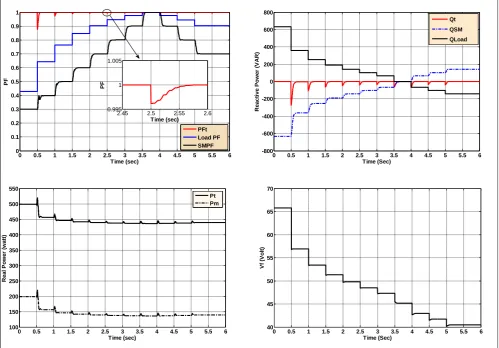
Fig.11: Simulation results for PF, real power, reactive power and field voltage variation vs time using FIS controller. Table 1: Synchronous machine inductance matrices.
ff cf bf af cf ac bf bc S b S ab af S ac S ab S a L L L L L Lc Ls L Ls L L Ls L L L L L L L L L L L L L bc ) 3 / 2 2 cos( ) 3 / 2 cos( ) cos( ) 3 / 2 cos( ) 2 cos( ) 2 cos( ) 3 / 2 2 cos( ) 3 / 2 cos( ) 2 cos( ) 2 cos( ) 3 / 2 2 cos( ) cos( ) 3 / 2 2 cos( ) 3 / 2 2 cos( ) 2 cos(
0 ) 3 / 2 sin( ) 3 / 2 sin( ) sin( ) 3 / 2 sin( ) 3 / 2 2 sin( 2 ) 2 sin( 2 ) 3 / 2 2 sin( 2 ) 3 / 2 sin( ) 2 sin( 2 ) 3 / 2 2 sin( 2 ) 3 / 2 2 sin( 2 ) sin( ) 3 / 2 2 sin( 2 ) 3 / 2 2 sin( 2 ) 2 sin( 2 cf bf af cf S S S bf S S S af S S S L L L L L L l L L L L L L L L d L d8.
ACKNOWLEDGMENTS
All thanks to my colleagues who help me to complete this work.
9.
REFERENCES
[1] Planning of Electric Power Distribution, Technical Principles, Published by Siemens AG 2016.
[2] T.W. Eberly and R.C. Schaefer, “Voltage versus VAr/ power-factor regulation on synchronous generators”, IEEE Transactions on Industry Applications ( Volume: 38, Issue: 6, Nov/Dec 2002, pp.1682 – 1687.
[3] Ramazan Bayindir, Ilhami Colak, Ersan Kabalci, Alper Gorgun, “PID controlled synchronous motor for power factor correction”, IEEE International Conference on Power Engineering, Energy and Electrical Drives, 2009.
[4] M.A. Abido and Y.L. Abdel-Magid, "A fuzzy basis function network for generator excitation control." IEEE Proceedings of The Sixth International Conference on Fuzzy Systems,3, pp. 1445-1450, 1997.
[5] E. Handschin, W. Hoffmann, F. Reyer, T. Stephanblome, U. Schlucking, D. Westermann and S.S. Ahmed, "A new method of excitation control based on fuzzy set theory" IEEE Transactions on Power Systems, 9(1),pp. 533-539, 1994.
[6] Rick Orman, “Power Factor Correction Solutions & Applications”, reference document, Eaton Corporation, 2012.
[7] Dr. Ahmed Nasser B. Alsammak, Abdulrazaq Ahmed M. Al-Nuaimy, “Transient Stability Improvement of
Multi-0 0.5 1 1.5 2 2.5 3 3.5 4 4.5 5 5.5 6
0 0.1 0.2 0.3 0.4 0.5 0.6 0.7 0.8 0.9 1 Time (sec) PF PFt Load PF SMPF
2.45 2.5 2.55 2.6
0.995 1 1.005
Time (sec)
PF
0 0.5 1 1.5 2 2.5 3 3.5 4 4.5 5 5.5 6
-800 -600 -400 -200 0 200 400 600 800 Time (Sec) R e a c ti v e P o w e r (V A R ) Qt QSM QLoad
0 0.5 1 1.5 2 2.5 3 3.5 4 4.5 5 5.5 6
100 150 200 250 300 350 400 450 500 550 Time (sec) R e a l P o w e r (w a tt ) Pt Pm
0 0.5 1 1.5 2 2.5 3 3.5 4 4.5 5 5.5 6
[image:9.595.108.495.452.574.2]machine Power Systems Using Modern Energy Storage Systems”, IJEIT, Volume 7, Issue 1, July 2017.
[8] Ahmed N. B. Al-Sammak, “A Fuzzy Logic Control of Synchronous Motor for Reactive Power Compensation”, PhD thesis, University of Mosul, 2017.
[9] I. Dobson and H.-D. Chiang, “Towards a theory of voltage collapse in electric power systems”, Systems and Control Letters, Vol. 13, 1989, pp. 253-262.
[10]M. F. Al-Kababji and Ahmed N. Al-Sammak, "Bifurcation and Voltage Collapse in the Electrical Power Systems", Al-Rafidain Engineering Journal Vol.13, No.1, 2005, pp.25-41.
[11]Dr. Ahmed Nasser B. Alsammak, Maan Hussein A. Safar, “Voltage stability margin improving by controlling power transmission paths”, IJEIT, Volume 7, Issue 1, July 2017.
[12]M. F. Al-Kababji and Ahmed N. Al-Sammak, "Adaptive Neuro-Fuzzy Inference System (ANFIS) Real Time Based Power Factor Control by Synchronous Machine", 1st EEC07, 26-28 June, 2007, FEEE, University of Aleppo-Syria, PS-5, pp.1-24.
[13]J.J. Buckley and E, Eslami, “An Introduction to Fuzzy Logic and Fuzzy Sets”, Physica-Verlag Heidelberg, Printed in Germany, 2002.
[14]Patrik Eklund, Lena Kallin and Tony Riissanen, ”Fuzzy Systems”, lecture notes, Department of Computing Science, Umeoa University, SE-901 87 Umeoa, Sweden, 2000.