The Evaluation of Software Solutions for Reliability
using Modified Musa’s Basic Execution Time Model
Terungwa Simon Yange
Department of Mathematics/Statistics/Computer Science
University of Agriculture, Makurdi
Onyekware U.
Oluoha
Department of Computer ScienceUniversity of Nigeria, Nsukka
ABSTRACT
Software systems have gained great significance for most organizations on an operational as well as a strategic level. Failures before delivery or more often changes in existing software systems are stochastic processes and it is important for programmers (or users) to predict reliability of software product they are developing (or using) in order to accept that as business risk. In this paper we have used the Modified Musa Basic Execution Time Model to show how to evaluate a healthcare solution called electronic Nursing Care Management System (eNCMS). We used black box testing to ascertain that the software achieved it basic functions. Five (5) patient records collected from Obafemi Awolowo University Teaching Hospital Complex (OAUTHC) were used during this evaluation and the outcome shows that the system achieved 75% reliability.
Keywords
Black box, reliability, healthcare, software reliability testing, testing.
1. INTRODUCTION
Software evaluation is the process of executing a program or system with the intent of finding errors. Or, it involves any activity aimed at evaluating an attribute or capability of a program or system and determining that it meets its required results. Software is not unlike other physical processes where inputs are received and outputs are produced. Where software differs is in the manner in which it fails. Most physical systems fail in a fixed (and reasonably small) set of ways. By contrast, software can fail in many bizarre ways [1].
Software reliability refers to the probability of failure-free operation of a system. It is related to many aspects of software, including the testing process [2]. Directly estimating software reliability by quantifying its related factors can be difficult. Testing is an effective sampling method to measure software reliability. Guided by the operational profile, software testing can be used to obtain failure data, and an estimation model can be further used to analyse the data to estimate the present reliability and predict future reliability [3]. Therefore, based on the estimation, the developers can decide whether to release the software, and the users can decide whether to adopt and use the software. Risk of using software can also be assessed based on reliability information.
Reliability Testing is very important, as it discover all the failures of a system and removes them before the system is deployed. This also determines the failure rate or failure intensity of a system. Software reliability is the measured in terms of failure intensity which is the number of failures per unit time. Reliability testing is related to many aspects of software in which testing process is included; this testing process is an effective sampling method to measure software
reliability. Robustness testing and stress testing are the variances of reliability testing. Robustness refers to how software component works under stressful environmental conditions. Robustness testing only watches the robustness problem such as machine crashes, abnormal terminations etc. [3].
Software reliability is one of the main factors to measure the quality of software. Since software errors cause spectacular failures in some cases, we need to measure the reliability factor to determine the quality of software product, predict reliability in the future, and use it for planning resources needed to fix failures. Software reliability models are applicable tools to analyze software in order to evaluate the reliability of software [1]. During the past twenty-five years, more than fifty different models have been proposed for estimating software reliability but many of software practitioners do not know how to utilize these models to evaluate their products. In this paper we will present a survey on different models of software reliability and their characteristics. We will propose taxonomy of different models and try to aid the comprehension of these models for practitioners, developers, and users. In the last section we apply some of these models on two different open source projects and compare the results.
2. BLACKBOX TESTING
This testing methodology looks at the available inputs for an application and what the expected outputs should result from each input. It is not concerned with the inner workings of the application, the process that the application undertakes to achieve a particular output or any other internal aspect of the application that may be involved in the transformation of an input into an output [4]. Most black-box testing tools employ either coordinate based interaction with the applications graphical user interface or image recognition. An example of a black box system would be a search engine. You enter text that you want to search for in the search bar, press “Search” and results are returned to you. In such a case, you do not know or see the specific process that is being employed to obtain your search results, you simply see that you provide an input-a search term-and you receive an output-your search results.
important to note that no amount of testing can unequivocally demonstrate the absence of errors and defects in a program. The beauty of black box testing is seen when the tester is not the programmer of the code and knows nothing about the structure of the code [5].
3. MUSA’S BASIC EXECUTION TIME
MODEL
The Musa’s Basic Execution Time Model is an example of a prediction model [3]. Prediction models are used to make software reliability predictions early in the development phase that help make software engineering decisions in the design stage. Musa’s Basic Execution Time Model is important to the field of software reliability because it was created by John Musa of AT&T Bell Laboratories who is often credited as the pioneer of software reliability[2]. Musa’s Basic Execution Time Model was one of the first software reliability models used to model reliability based on the execution time of software components instead of the calendar time components are in use. Since the time between failures can be expressed in terms of CPU (central processing unit) time, Musa’s Basic Execution Time Model can accurately indicate the actual stress on the software system. Musa’s Basic Execution Time Model calculates the reliability of a software system using the Poisson distribution. The model assumes the execution time between failures has piecewise exponential distribution, the hazard rate of a single fault is constant, faults are removed with certainty and reoccurring failures caused by a single fault are not counted [5]. The data required to implement Musa’s Basic Execution Time Model include the time elapsed between software failure and the actual calendar time the software was in use. Musa’s Basic Execution Time Model is useful when predicting why a software system might fail when deployed. Musa’s Basic Execution Time Model has been used to calculate the reliability of land line telephone software. Musa’s Basic Execution Time Model is a good reliability model to use when the model is based on sound assumptions and a simple model is both desired and achievable. Because of the above-mentioned reasons, the simplicity and ease of use, this model is employed in this research to evaluate the system.
Since in this case, the focus is on reliability testing, both white box and black box testing techniques were employed, the white box testing was done by the developer and the result was evaluated using the extended or modified Musa’s software reliability model which is discussed in this section. The black box testing was done by some registered nurses and the result was also evaluated using extended Musa’s model. In both cases of the testing, the extent to which the system could go without failure was determined.
Since the system is made up of different modules or functional components, testing these different components gives the most accurate result for the reliability of the system since the testing leads to the dynamic verification of the behaviour of each module on a finite set of the test cases which are suitably selected from the usually infinite executions domain, against the specified expected behaviour. The testing effort is divided into test case generation, test execution, test evaluation. To reduce the cost of testing process, efficient test case generation technique is required. The reliability of the functional components of the system was then computed using the modified Musa’s Basic Execution Time Model [1]. This model was chosen because it is very simple to use and can determine the maximum errors in the system without taking much time.
With this model, it is possible to predict the final number of failures (usually denoted by v0 ) that will be detected in the future, after the system delivery. This software reliability growth models assume that software failures occur as a random non-homogeneous Poisson process (NHPP) and it is possible to evaluate Markov models from NHPP models and predict system’s reliability by solving state equations with numerical integration [1]. The model used in this section called modified Musa Basic execution time is is based on the following basic assumptions where the cumulative number of failures experienced at time t is N(t) [1]:
i. There are no failures to begin with (for t=0,N(t)=N(0)=0)
ii. The failures are independent, the number of failures experienced during the interval (t, t+h) is independent of the past history, N(t)
iii. The probability that a failure will occur during (t, t+h) is:
–
(0.1)
Where o(h) is negligible when h is small. There are no simultaneous failures.
iv. The probability that more than one failure will occur during (t, t+h) is o(h)
– (0.2)
Failure rate is time dependent. This describes a Non-Homogeneous Poisson Process where λ is a failure rate and varies with time. There are different NHPP models connected with the representation of λ(t) function. The mean value of failure distribution is:
(0.3)
Where μ(t) is the expected number of cumulative failures at time t. In order to derive this model, it is assumed that we can
estimate the expected number of total failures can be determined. It can be assumed that the initial failure rate can be predicted if n is the mean cumulative number of failures experienced at some point in the testing process, then the basic failure rate is expressed as:
(0.4)
Where: = initial failure rate, = average number of failures
experienced at a given point in time = total number of failures in the program, detected if given infinite time. In this
model, the failure rate
is a linear function of the experienced software failure. The rate of change of
can be determined by taking the derivative:
(0.5)
If the decrement of the software failure rate per failure is denoted as:
Then the failure rate is expressed as:
(0.7)
Since the mean number of software failures is experienced as a function of the execution time t, it is:
(0.8)
Since μ(t) is the time integral of
it follows that
is the derivate of μ(t). Then the equation can be rewritten as:
(0.9)
With solving of the above differential equation for
it is obtained:
–
(0.10)The failure rate can be obtained by:
(0.11)
In either case, failure rate function decreases exponentially to 0 and the initial failure rate is evaluated (at t=0) as:
(0.12)
In addition to the basic execution time model described in this section, many others have been proposed in the past. One with the widest distribution among the software reliability models was deployed by John Musa during his work at AT&T Bell Laboratories (Musa, 1993). Including the standard assumptions above, the basic assumptions for Musa’s basic execution time model are:
i. The cumulative number of failures by time t, follows a Poisson process with mean value function μ(t)= (1 – exp [−βt]) , where , β>0. The mean value function is such that the expected number of failure occurrences for anytime period is proportional to the expected number of undetected faults at that time.
ii. Used model is a finite failure model.
Suppose n observed failures of the software system at times
, ,…, and from the last failure time an additional time of x (x>=0) elapsed without failure ( (
is therefore the total time the software component has been observed since the start). Using the model assumptions, the likelihood function (Musa, 1993) is obtained as:
(0.13)
The maximum likelihood estimates (MLEs) [1] of and β are obtained as the solutions to the following pair of equations:
(0.14)
(0.15)
Once the estimates of and β are obtained, it is possible to use the invariance property of the MLEs to estimate other reliability measures like reliability function, hazard rate, failure intensity function etc.. This approach is then use to evaluate our system.
4. CASE STUDY: THE ELECTRONIC
NURSING CARE MANAGEMENT
SYSTEM
This application is a comprehensive, integrated information system designed to manage the patient care, administrative, financial and legal aspects of nursing. The solution can also be used to monitor staffing levels and achieve more cost-effective staffing. Nurses could also use it for admission information, care plan and all relevant nursing notes. All important data is securely stored and can be retrieved when required. All these features in this system ultimately lead to a reduction in planning time and better assessments and evaluations.
being the blueprint of this process is generated as well. The assessment phase in this system is based on the Gordon’s functional health patterns [11]. The Nursing History Module: This keeps the archive of all the activities that are carried out on the system.
The NNN Linkage module creates the library for nursing diagnoses, outcomes and interventions. During the development of the care plan, reference is made to this module to get the diagnoses, outcomes and interventions. The nursing process module enables the nurse to create the nursing care plan. This module is central to all the other modules. The history module is the module that keeps track of all the activities of the nurses during the implementation of the nursing process. The reliability of these components implies the reliability of the whole system.
The evaluation of this system was carried out in two phases. First, the functional components of the system were tested with some existing care plans to see if the output tallies with those care plans; any deviation from that result into a failure. Therefore, failure here is not system failure or error but deviation from the expected output. The functional components and their respective functions are shown in table 1. In the second phase, the failure log resulting from the testing is evaluated using the reliability model described above and the result is represented on graphs.
Software reliability is therefore centred around software faults, their effect on the system and the remaining number of faults, system failures, the way of detecting failures, time between failures and failure rates (or failure intensities), as well as the confidence in the performed estimates. Identifying faults and removing them leads to the decrease of the system failure rate and the increase of the system reliability with time. The cumulative number of errors detected and corrected increases with the passage of time. This makes the software reliability curve to look like a demand curve. In order to evaluate this system, the model described in section 3 will be used. The standard assumptions for this model are:
i. The rate of fault detection is proportional to the current fault content of software.
ii. The fault detection rate remains constant over the intervals between fault occurrences
iii. A fault is corrected instantaneously without introducing new faults into the software
iv. The software is operated in a similar manner as that in which reliability predictions are to be made v. Every fault has the same chance of being
encountered within a severity class as any other fault in that class
vi. The failures, when the faults are detected, are independent
The system was tested using five (5) patient data collected from Obafemi Awolowo University Teaching Hospital Complex (OAUTHC), Ile-Ife, Nigeria.
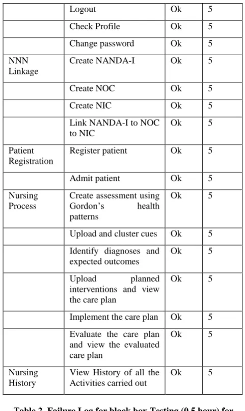
Table 1. Test Cases for Black box Testing
Module Function Result No of
Runs
User Management
Create Users Ok 5
Login Ok 5
Logout Ok 5
Check Profile Ok 5
Change password Ok 5
NNN Linkage
Create NANDA-I Ok 5
Create NOC Ok 5
Create NIC Ok 5
Link NANDA-I to NOC to NIC
Ok 5
Patient Registration
Register patient Ok 5
Admit patient Ok 5
Nursing Process
Create assessment using Gordon’s health patterns
Ok 5
Upload and cluster cues Ok 5
Identify diagnoses and expected outcomes
Ok 5
Upload planned interventions and view the care plan
Ok 5
Implement the care plan Ok 5
Evaluate the care plan and view the evaluated care plan
Ok 5
Nursing History
View History of all the Activities carried out
[image:4.595.307.548.69.472.2]Ok 5
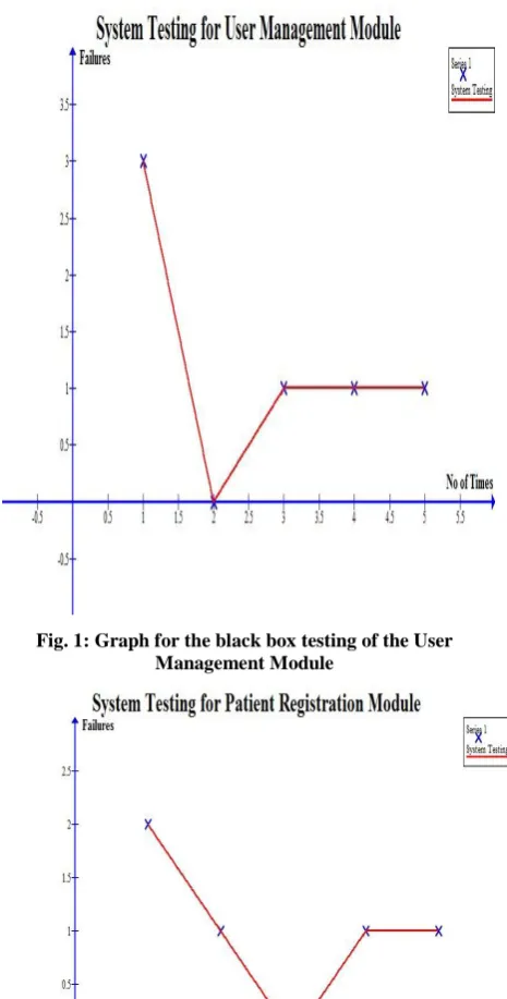
Table 2. Failure Log for black box Testing (0.5 hour) for User Management Module
No of Time New Failure Detected
1 3
2 0
3 1
4 1
[image:4.595.311.548.490.608.2]5 1
Table 3. Failure Log for black box Testing (0.5 hour) for Patient Registration Module
No of Time New Failure Detected
1 2
2 1
3 0
4 1
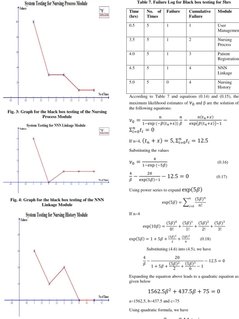
Table 4. Failure Log for black box Testing (3 hours) for Nursing Process Module
No of Time New Failure Detected
1 10
2 3
3 3
4 1
[image:5.595.52.288.93.215.2]5 1
Table 5. Failure Log for black box Testing (0.5 hours) for NNN Linkage Module
No of Time New Failure Detected
1 4
2 0
3 1
4 1
5 1
Table 6. Failure Log for black box Testing (0.5 hours) for Nursing History Module
No of Time New Failure Detected
1 3
2 1
3 2
4 0
5 0
The Fig. 1, Fig. 2, Fig. 3, Fig. 4 and Fig. 5; derived their values from Table 2, Table 3, Table 4, Table 5 and Table 6 respectively. Looking at the graphs for the black box testing of the modules, they all slope downward from left to right just like a demand curve. This is because as the software is tested, faults are identified and corrected which reduces the number of faults present in the system thereby making the curve to start from a higher frequency and slope down to a lower one. On the other hand, as these faults are identified and corrected, new faults are introduced which make curve to move up and down which makes the curves not to be smooth.
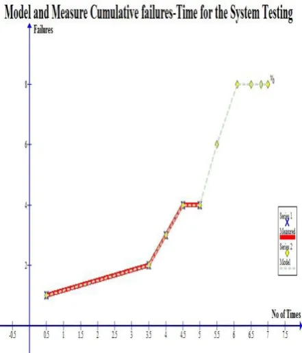
[image:5.595.315.554.380.591.2]The cumulative number of errors is a function that increases with time and asymptotically approaches the total number of errors V0. By systematically detecting failures and removing faults, it is possible to achieve the required system mean time to failure (MTTF). The curve for the cumulative failure rate for the black box testing of the five functional modules of the system is shown in fig. 6. Here, we arrived at V0 after testing all the modules several times and its value is 8. This is because no new failure was detected after this was achieved. This shows that the software is very reliable.
Fig. 1: Graph for the black box testing of the User Management Module
[image:5.595.49.287.400.515.2]Fig. 3: Graph for the black box testing of the Nursing Process Module
Fig. 4: Graph for the black box testing of the NNN Linkage Module
Fig. 5: Graph for the black box testing of the Nursing History Module
Table 7. Failure Log for Black box testing for 5hrs
Time (hrs)
No. of Times
Failure Cumulative Failure
Module
0.5 5 1 1 User
Management
3.5 5 1 2 Nursing
Process
4.0 5 1 3 Patient
Registration
4.5 5 1 4 NNN
Linkage
5.0 5 0 4 Nursing
History
According to Table 7 and equations (0.14) and (0.15), the maximum likelihood estimates of and β are the solution of the following equations:
If n=4,
Substituting the values
(0.16)
(0.17)
Using power series to expand
If n=4
(0.18)
Substituting (4.6) into (4.5), we have
Expanding the equation above leads to a quadratic equation as given below
a=1562.5, b=437.5 and c=75
Using quadratic formula, we have
[image:6.595.307.519.308.632.2] [image:6.595.58.273.505.724.2]But cannot be negative, therefore,
, substituting the value of in (0.16), we have
But the total number of failures cannot be a fraction, therefore, the value of our will be 8 instead of 7.9457.
With these results we can expect final number of the failures that are caused by errors in software design.
If the values of β and are known then is possible to draw model graph of cumulative failures with using of equation (0.10).
–
Comparison of cumulative failures between model and measured values is good during validation phase. It is obvious that the testing time was too short to achieve the predicted final number of failures. According to the model prediction for the presented case, three failures could be expected after this period as the difference between predicted value for
[image:7.595.59.280.441.699.2]and the final number of measured failures from Table 7. In the presented case, it was decided that achieved reliability of three predicted future failures is good enough for the developed product. The graph for this is shown in Fig. 6.
Fig. 6: Graph of Cumulative Failures (Comparison between measured and model)
In evaluating the system using black box testing, a total of six (6) errors were detected and using the model, two (2) more errors were uncovered; and because these two (2) errors were not corrected during the actual testing, we have a reliability of 0.75 (75%). With the result of these two (2) testing methods, it shows that the software is very reliable.
5. CONCLUSION
In this paper, we used the Musa’s basic execution time model which was sufficient for reliability modelling of the eNCMS presented. This model was able to give predictive information (expected number of future failures) about the system. It is also possible to apply described model to other problems such as the optimal software release problem.
6. ACKNOWLEDGEMENTS
We would like to thank all the members of Health Information System Research Group, Department of Computer Science and Engineering, Obafemi Awolowo University, Ile-Ife for their helpful comments on the manuscript and for significant logistical supporting the design and conduct of the research.
7. REFERENCES
[1] Urem, F. and Mikulic, Z. 2010. Developing operational profile for ERP software module Reliability Prediction. 2010 Proceedings of the 33rd International Convention, Department of management, College of Sibenik, Crotia, 409-413.
[2] Pai, G. 2002. A Survey of Software Reliability Models. Department of ECE University of Virginia, VA,1-12.
[3] Musa, J. D. 1993. Operational Profiles in Software Reliability Engineering. IEEE Software Magazine, 14-32.
[4] Koziolek, H. 2005. Operational Profiles for Software Reliability. Seminar “Dependability Engineering”, 1-17.
[5] Lyu, M. R. 2007. Software Reliability Engineering: A Roadmap. Future of Software Engineering, 2007. FOSE ’07, 153-170.
[6] Johnson, M. 2006. Linking NANDA-I, NOC, and NIC. International Journal of Nursing Terminologies & Classifications, 17(1): 39-40.
[7] NANDA International (Eds.). 2009. Nursing Diagnoses: Definition & Classification, 2009-2011. Oxford: Wiley-Blackwell.
[8] NANDA International (Eds.). 2012. Nursing Diagnoses: Definition & Classification, 2012- 2014. Oxford: Wiley-Blackwell.
[9] Moorhead, S., Johnson, M., Maas, M., and Swanson, E. (Eds.). 2008. Nursing outcomes classification (NOC) (4th ed.). St. Louis, MO: Mosby.
[10] Bulechek, G. M., Butcher, H. and Dochterman, J. M. (Eds.). 2008. Nursing Interventions Classification (NIC). (5th ed.). St. Louis, MO: Mosby.