The Variability of
P
-Values
Dennis D. Boos Department of Statistics North Carolina State University
Raleigh, NC 27695-8203 [email protected]
August 15, 2009
NC State Statistics Departement Tech Report # 2626
Summary
P-values are used as evidence against a null hypothesis. But is it enough to report a p -value without some indication of its variability? Bootstrap prediction intervals and standard errors on the log scale are proposed to complement the standard p-value.
1
Introduction
Good statistical practice is to report some measure of variability or reliability for important quantities estimated, that is, for estimates of the primary parameters of interest. Thus if the population mean µ is a key focus and estimated by the sample mean Y from a simple iid sample Y1, . . . , Yn, one should also report the standard errors/√n and/or a confidence interval for µ. One could carry the logic forward and say that standard errors should also be reported for s/√n or for the endpoints of the confidence interval, but most would agree that standard errors and confidence interval endpoints are secondary measures that usually do not require standard errors themselves.
Ap-value is simply the probability of obtaining as extreme or a more extreme result than found in observed data Y, where the probability is computed under a null hypothesis H0. Thus, for example, if T is a statistic for which large values suggest rejection of H0, then the
p-value is justP(T ≥T(Y)|Y), whereT(Y) is the value ofT computed from the observed data, considered fixed, andT is an independent generation ofT under H0.
Arep-values primary measures and deserving of some focus on their variability? Perhaps the answer has to do with how much they are emphasized and relied upon, but often p -values are thought of as important measures of evidence relative toH0. In that role, it seems plausible to understand something of their variability.
I usep-values as a quick and dirty method for detecting statistical significance, i.e., true “signals” in the presence of noise. In recent years, I have been promoting the use of exact
p-values because there seems to be no reason to rely on mathematical approximation when exact methods are available. For example, rank statistics and categorical data analyses are often built on permutation methods that allow conditionally exact p-values. Statistical computing packages like StatXact have led the way in making these p-values available, at least by Monte Carlo approximation.
deeply about the problem. I get excited when I see a p-value like 0.002. But what if an identical replication of the experiment could lead top-values that range from 0.001 to 0.15? That is not so exciting.
So, how should one measure and report the variability of a p-value? This is not as obvious as it first seems. For continuous T under a simpleH0, thep-value has a uniform(0,1) distribution. But under an alternative Ha, the logarithm of the p-value is asymptotically normal (see Lambert and Hall, 1982, and Example 2 below). Thus, the p-value can have a quite skewed distribution under Ha, and simply reporting an estimate of its standard deviation is not very satisfying for those situations. One solution is to get comfortable with the log(p-value) scale and just report a bootstrap or jackknife standard error on that scale. (Actually, I prefer the base 10 logarithm as I will explain later.)
But because most people are used to thinking on thep-value scale and not its logarithm, I propose a prediction interval for the p-value composed of modified quantiles from the bootstrap distribution of the p-value. This bootstrap prediction interval captures the p -value from a new, independent replication of the experiment. Mojirsheibani and Tibshirani (1996) and Mojirsheibani (1998) developed these bootstrap intervals for a general statistic computed from a future sample. One of their intervals, the nonparametric bias-corrected (BC) bootstrap prediction interval, is briefly described in Section 3 and used in the examples in Section 2 and in the Monte Carlo experiments in Section 4.
2
Examples
Example 1. To decide if consumers will be able to distinguish between two types of a food product, n = 50 sets of three samples are prepared, with half of the sets consisting of two samples from type A and one from type B, and half of the sets with two samples from Type B and one from Type A. Fifty randomly chosen judges are asked to tell which samples of their set are from the same type. The hypotheses areH0 :π= 1/3 (random guessing) versus
0.011, and the normal approximation without continuity correction is 0.006. Should we care that the normal approximation overstates the significance by roughly a factor of 2? Probably not. Let’s see why.
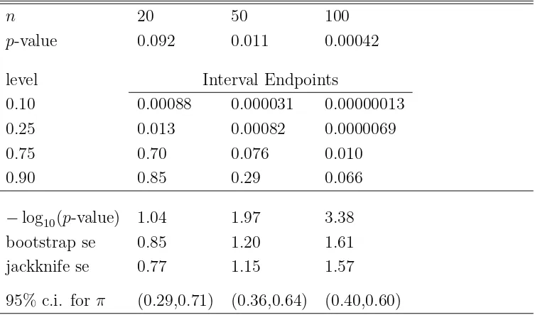
Table 1 givesp-value prediction intervals whenπb= 1/2 andn= 20, 50, and 100 using the bootstrap prediction interval method described in Section 3. For example, an 80% prediction interval whenn = 50 is (0.000031, 0.29) Thus, a replication of the experiment will result in a
p-value lying in this interval 80% of the time. The related 90% lower and upper bounds are 0.000031 and 0.29, respectively. The central 50% interval is (0.00082, 0.076), encompassing values much farther from the exact p-value = 0.011 than the normal approximation p-value = 0.006.
Table 1: Bootstrap prediction interval endpoints for a future p-value and standard errors for the base 10 logarithm of the p-value. Binomial test of H0 :π= 1/3 versus Ha:π >1/3,bπ = 1/2.
n 20 50 100
p-value 0.092 0.011 0.00042
level Interval Endpoints
0.10 0.00088 0.000031 0.00000013
0.25 0.013 0.00082 0.0000069
0.75 0.70 0.076 0.010
0.90 0.85 0.29 0.066
−log10(p-value) 1.04 1.97 3.38
bootstrap se 0.85 1.20 1.61
jackknife se 0.77 1.15 1.57
95% c.i. for π (0.29,0.71) (0.36,0.64) (0.40,0.60)
Bootstrap endpoints and standard errors computed from binomial(n,πb) without resampling. Endpoints are one-sided bounds. Intervals are formed by combining symmetric endpoints (0.10,0.90) or (0.25,0.75).
significance results used in many subject matter journals: one star * forp-values ≤0.05, two stars ** for p-values ≤ 0.01, and three stars *** for p-values ≤ 0.001. If we replace 0.05 by 0.10, then the rule is: * if −log10(p-value) is in the range [1,2), ** for the range [2,3), and *** for the range [3,4). In fact, looking at the standard errors for −log10(p-value) in Table 1, it might make sense to round the−log10(p-value) values to integers. That would translate into rounding the p-values: 0.092 to 0.10, 0.011 to 0.01, and 0.00042 to 0.001. Thus, taking into account the variability in −log10(p-value) seems to lead back to the star (*) method. To many statisticians this rounding seems information-robbing, but this opinion may result from being unaware of the variability inherent in p-values.
A standard complement to thep-value is a 95% confidence interval for π. Withπb= 1/2, these intervals for n = 20, 50, and 100 are given at the bottom of Table 1. They certainly help counter over-emphasis on smallp-values. For example, atn = 50 the confidence interval is (0.36, 0.64), showing that the trueπ could be quite near the null value 1/3.
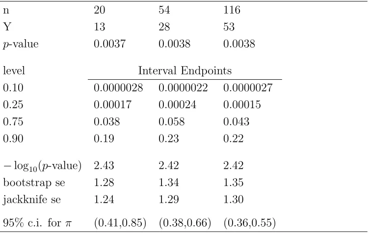
Table 2 illustrates the prediction intervals when the p-value is held constant near 0.0038, but n changes from 20 to 54 and to 116. These results suggest that the same p-value at different sample sizes has a somewhat similar variability and repeatability. For example, with ap-value around 0.0038 for these situations, the 75% upper bounds are roughly similar: 0.038, 0.058, and 0.063. Note also that the bootstrap and jackknife standard errors in Table 2 for the base 10 logarithm of the p-value are nearly the same. The confidence intervals for
π, though, are quite different in these experiments because they are centered differently.
Example 2. Consider samples of sizenfrom a normal distribution with meanµand variance
σ2 = 1 and the hypotheses H
0 :µ = 0 vs. Ha : µ > 0. If one assumes that the variance is known, then Lambert and Hall (1982, Table 1) give that the p-values fromZ =√nY /σ for
µ >0 in Ha satisfy √
n
log(p-value)
n +µ
2/2
d
−→N(0, µ2), as n → ∞, (1)
or equivalently that −log(p-value)/n is asymptotically normal with asymptotic mean µ2/2 and asymptotic variance µ2/n. This asymptotic normality implies that
Table 2: Bootstrap prediction interval endpoints for a future p-value and standard errors for the base 10 logarithm of the p-value. Binomial test of H0 :π= 1/3 versus Ha:π >1/3.
n 20 54 116
Y 13 28 53
p-value 0.0037 0.0038 0.0038
level Interval Endpoints
0.10 0.0000028 0.0000022 0.0000027
0.25 0.00017 0.00024 0.00015
0.75 0.038 0.058 0.043
0.90 0.19 0.23 0.22
−log10(p-value) 2.43 2.42 2.42
bootstrap se 1.28 1.34 1.35
jackknife se 1.24 1.29 1.30
95% c.i. for π (0.41,0.85) (0.38,0.66) (0.36,0.55)
Bootstrap endpoints and standard errors computed from binomial(n,πb) without resampling. Endpoints are one-sided bounds. Intervals are formed by combining symmetric endpoints (0.10,0.90) or (0.25,0.75).
A similar result obtains in the unknown variance case where the usualt=√nY /sreplacesZ, but the constants are more complicated. For example, the asymptotic mean is (1/2) log(1 +
µ2/2), in place of µ2/2, and the asymptotic variance is µ2(1 +µ2)−2(1 +µ2/2) in place ofµ2.
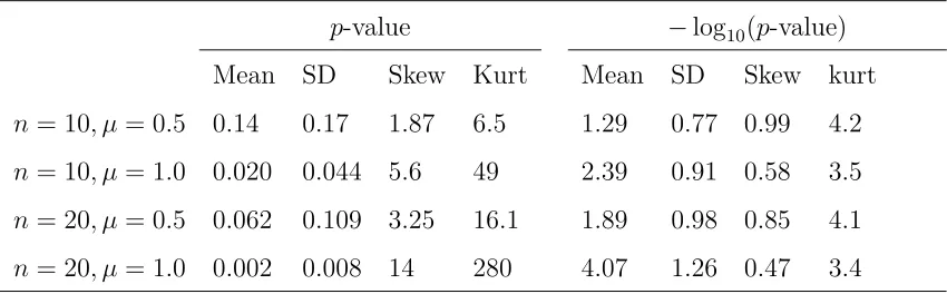
Table 3 illustrates the asymptotic normality of−log10(p-value) for the one-samplet-test. Thep-values themselves are clearly not normally distributed because the third moment ratio Skew and the fourth moment ratio Kurt given by E{X−E(X)}k/[E{X−E(X)}2]k/2 for
k = 3 and k = 4, are not near their normal distribution values of 0 and 3, respectively. Although the Skew values for −log10(p-value) are not close to 0, the trend from n = 10 to
n= 20 is down, and the values at n= 50 (not displayed) are 0.60 and 0.33, respectively, for
µ= 0.5 and µ= 1.0.
In-Table 3: Distribution summaries for the t-test p-value and −log10(p-value) for the normal location problem, H0 :µ= 0 versus Ha :µ >0,σ = 1 unknown.
p-value −log10(p-value)
Mean SD Skew Kurt Mean SD Skew kurt
n= 10, µ= 0.5 0.14 0.17 1.87 6.5 1.29 0.77 0.99 4.2
n= 10, µ= 1.0 0.020 0.044 5.6 49 2.39 0.91 0.58 3.5
n= 20, µ= 0.5 0.062 0.109 3.25 16.1 1.89 0.98 0.85 4.1
n= 20, µ= 1.0 0.002 0.008 14 280 4.07 1.26 0.47 3.4
Based on 10,000 Monte Carlo samples. Skew and Kurt are the moment ratios, E{X−E(X)}k/[E{X−E(X)}2]k/2, for k = 3 andk = 4, respectively. Standard errors of entries are in the last decimal displayed or smaller.
verting the asymptotic pivotal statistic implied by (1) leads to the asymptotic prediction interval
exp−z1−α/2
√
nµ−nµ2/2 , expz1−α/2
√
nµ−nµ2/2 , (3)
where z1−α/2 is the 1−α/2 quantile of the standard normal. Substituting the sample mean
Y forµthen yields a possible competitor to the bootstrap intervals. Unfortunately, unlessY
is fairly large, the right endpoint is often larger than one, and the interval is not informative.
However, the result (1) seems to support the observation from Table 2 that equalp-values from different experiments with different sample sizes have similar prediction intervals. That is, letting Pn=p-value and setting µ2/2 = −log(Pn)/n from (2) and solving for µ yields b
µ={−2 log(Pn)/n}1/2. Then, plugging bµinto (3) yields
expn−z1−α/2{−2 log(Pn)}
1/2
+ log(Pn)o, expnz1−α/2{−2 log(Pn)}
1/2
+ log(Pn)o,
(4)
and sample sizes do not appear in the endpoint expressions except throughPn.
The general result in Lambert and Hall (1982) for a variety of testing procedures about
asymp-totic variance nτ2(µ), where the functions c(·) and τ2(·) depend on the procedure. Thus, the asymptotic mean is proportional to n, and the asymptotic standard deviation is pro-portional to √n. In Table 3, these results are crudely supported by the ratio of means for −log10(p-value), 1.89/1.29=1.5 forµ= 0.5 and 4.07/2.39=1.7 for µ= 1.0 where 20/10 = 2. Similarly, the ratios of standard deviations 0.98/0.77=1.3 and 1.26/0.91=1.4 are not far from p
20/10 = 1.4.
Example 3. Miller (1986, p. 65) gives data from a study comparing partial thromboplastin times for patients whose blood clots were dissolved (R=recanalized) and for those whose clots were not dissolved (NR):
R 41 86 90 74 146 57 62 78 55 105
46 94 26 101 72 119 88
NR 34 23 36 25 35 23 87 48
The exact two-sided Wilcoxon Rank Sump-value is 0.0014 and the normal approximation without continuity correction is 0.0024. A 50% prediction interval for an exact future p -value based on B = 999 resamples is (0.00007, 0.018) and for the approximate p-value is (0.00037, 0.020). The value of −log10(p-value) for the exact p-value is 2.84 with bootstrap standard error 1.27 and jackknife standard error 1.31, thus suggesting one round 2.84 to 3 and the p-value from 0.0014 to 0.001. Similarly, the value of−log10(p-value) for the normal approximation p-value is 2.61 with bootstrap standard error 0.84 and jackknife standard error 0.89, leading to rounding 2.61 to 3 and 0.0024 to 0.001.
Example 4. The following data, found in Larsen and Marx (2001, p. 15), are the ordered values of a sample of width/length ratios of beaded rectangles of Shoshoni indians:
.507 .553 .576 .601 .606 .606 .609 .611 .615 .628 .654 .662 .668 .670 .672 .690 .693 .749 .844 .933
based on B = 999 resamples. So the p-value from a second sample from this population could easily be higher than the observed 0.012, but we expect it to be less than 0.094 with confidence 0.75. The value of −log10(p-value) is 1.93 with bootstrap standard error 1.23, again suggesting one round 1.93 to 2 and the p-value from 0.012 to 0.01.
3
Bootstrap Prediction Intervals
Consider an iid random sampleY1, . . . , Ynand an independent “future” iid sampleX1, . . . , Xm from the same population, and statistics Tn and Tm computed from these samples, respec-tively. If n = m, then Tn and Tm have identical distributions. Mojirsheibani and Tib-shirani (1996) and Mojirsheibani (1998) derived bootstrap prediction intervals from the Y
sample that contain Tm with approximate probability 1−α. Here I briefly describe their corrected (BC) interval. Mojirsheibani and Tibshirani (1996) actually focused on bias-corrected accelerated (BCa) intervals, but I am using the BC intervals for simplicity.
Let Y∗
1, . . . , Yn∗ be a random resample taken with replacement from the set (Y1, . . . , Yn), i.e., a nonparametric bootstrap resample, and let Tn(1) be the statistic calculated from the
resample. Repeating the process independently B times results in Tn(1), . . . , Tn(B). Let KBb
be the empirical distribution function of theseTn(i), and letηBb (α) be the related αth sample
quantile. Then, the 1−α bias-corrected (BC) bootstrap percentile prediction interval for
Tm is
{bηB(α1), ηBb (1−α2)}, (5)
whereα1 = Φ zα/2(1 +m/n)1/2+zb0(m/n)1/2
, 1−α2 = Φ z1−α/2(1 +m/n)
1/2+ b
z0(m/n)1/2
In practice, I suggest using B = 999 as in Examples 3 and 4, but B = 99 was used for some of the simulations in Section 4 (where only B = 999 results are reported), and the intervals performed reasonably well. For the binomial example, I calculated the endpoints of the intervals directly from the binomial distribution, i.e., from the exact bootstrap distri-bution. Note that in this paper I am using nonparametric bootstrap methods, resampling directly from the observed data. But for binomial data that can be strung out as a sequence of Bernoulli random variables, directly resampling of the Bernoulli data is equivalent to resampling from a binomial(n,πb).
Where does the factor (1 +m/n)1/2 come from? The easiest way to motivate it is to consider the following pivotal statistic used to get a prediction interval for the sample mean from a future sample, Tm =X, with known variance σ2,
Y −X
σ
1
n +
1
m
1/2.
Inverting this statistic gives the prediction interval
Y −σm1/2(1 +m/n)1/2z1−α/2, Y +σm
1/2(1 +m/n)1/2z 1−α/2
,
and the factor (1 +m/n)1/2 appears naturally due to taking into account the variability of bothY and X.
4
Monte Carlo Results
In this section I give results on empirical coverage and average length of the BC prediction intervals described in Section 3 for situations related to Examples 1 and 4 of Section 2 (Tables 4 and 5) and some results on the bootstrap and jackknife standard errors related to Examples 1,2, and 4 (Table 6). In each situation of Tables 4 and 5, 1000 Monte Carlo “training” samples are generated as well as a corresponding independent “test” sample. For each training sample, the intervals are computed and assessed as to whether they contain the
for all cases displayed in Table 5, butB = 99 was also used and gave similar results for most cases. All computations were carried out in R.
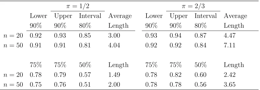
Table 4: Empirical coverages and lengths of bootstrap prediction intervals for p-values from the binomial test of H0 :π = 1/3 versus Ha:π > 1/3.
π= 1/2 π = 2/3
Lower Upper Interval Average Lower Upper Interval Average
90% 90% 80% Length 90% 90% 80% Length
n= 20 0.92 0.93 0.85 3.00 0.93 0.94 0.87 4.47
n= 50 0.91 0.91 0.81 4.04 0.92 0.92 0.84 7.11
75% 75% 50% Length 75% 75% 50% Length
n= 20 0.78 0.79 0.57 1.49 0.78 0.82 0.60 2.42
n= 50 0.75 0.76 0.51 2.00 0.78 0.78 0.56 3.65
Monte Carlo replication size is 1000. Bootstrap estimates are based on binomial(n,bπ). Standard errors for coverage entries are bounded by 0.016. Average length is on the base 10 logarithm scale; standard errors are a fraction of the the last decimal given. “Lower” and “Upper” refer to estimated coverage probabilities for intervals of the form (L,1] and [0,U), respectively.
Table 4 is for the binomial sampling of Example 1. Two alternatives are covered, π= 1/2 and π= 2/3 withH0 :π = 1/3 as in the example. Here we see excellent coverage properties for even n = 20. Because of the discreteness, the endpoints of the intervals were purposely constructed from the binomial(n,bπ) (equivalent to B = ∞ resamples) to contain at least probability 1−α. This apparently translated into slightly higher than nominal coverage. The average interval lengths are on the base 10 logarithm scale because interval lengths on the two sides of the p-value are not comparable (e.g., in Table 1 for n = 50 compare 0.011−0.000031 to 0.29−0.011).
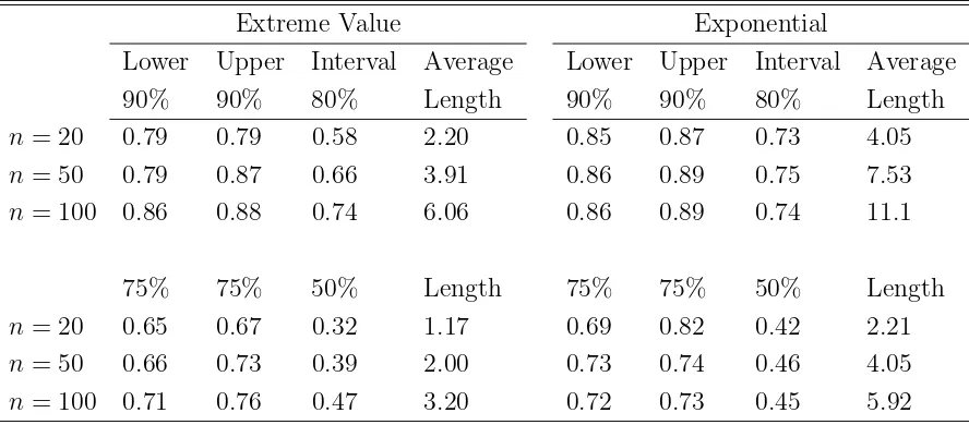
distribution, the coverages are not very good for small sample sizes but are reasonable by
n = 100. For the exponential distribution, the coverages are not too bad for even n = 20, but the improvement is very minor for larger sample sizes up to n = 100. The convergence to normality of the Anderson-Darling statistic under an alternative is very slow and is likely driving the the slow convergence of the coverage of the prediction intervals.
Table 5: Empirical coverages and lengths of bootstrap prediction intervals forp-values from the Anderson-Darling test for normality
Extreme Value Exponential
Lower Upper Interval Average Lower Upper Interval Average
90% 90% 80% Length 90% 90% 80% Length
n= 20 0.79 0.79 0.58 2.20 0.85 0.87 0.73 4.05
n= 50 0.79 0.87 0.66 3.91 0.86 0.89 0.75 7.53
n= 100 0.86 0.88 0.74 6.06 0.86 0.89 0.74 11.1
75% 75% 50% Length 75% 75% 50% Length
n= 20 0.65 0.67 0.32 1.17 0.69 0.82 0.42 2.21
n= 50 0.66 0.73 0.39 2.00 0.73 0.74 0.46 4.05
n= 100 0.71 0.76 0.47 3.20 0.72 0.73 0.45 5.92
Monte Carlo replication size is 1000. Bootstrap replication size is B = 999. Standard errors for coverage entries are bounded by 0.016. Average length is on the base 10 logarithm scale, standard errors are a fraction of the the last decimal given. “Lower” and “Upper” refer to estimated coverage probabilities for intervals of the form (L,1] and [0,U), respectively.
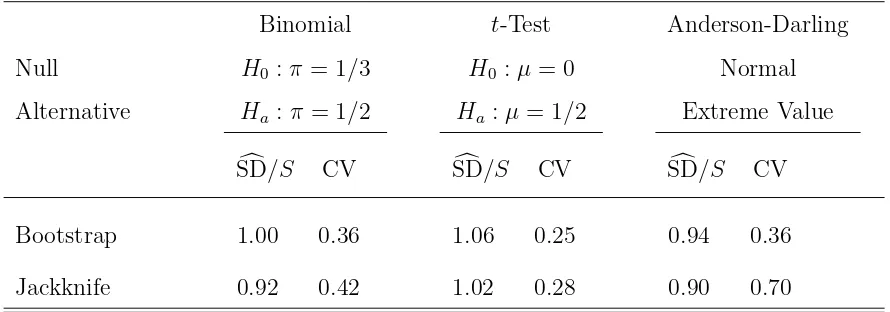
Table 6 briefly assesses the bias and variation of the bootstrap and jackknife standard errors for−log10(p-value) forn= 20 for one alternative for the tests from Examples 1, 2, and 4. Both bootstrap and jackknife are relatively unbiased as evidenced by the ratios SDc/S
Monte Carlo sample standard deviation of the standard errors divided by the Monte Carlo average of the standard errors. Other alternatives gave similar results with larger sample sizes showing improved results. For example, for the Anderson-Darling test with extreme value data at n= 50, the ratiosSDc/S are 0.98 and 0.95, respectively, and the coefficients of variation are 0.42 and 0.57.
Table 6: Bias and coefficient of variation (CV) of bootstrap and jackknife standard errors of −log10(p-value) for the binomial test, t-Test, and Anderson-Darling goodness-of-fit test for normality when n = 20. Bias assessed by the ratio of SD=Monte Carlo average ofc the bootstrap and jackknife standard errors for −log10(p-value) to S=Monte Carlo sample standard deviation of −log10(p-value).
Binomial t-Test Anderson-Darling
Null H0 :π = 1/3 H0 :µ= 0 Normal
Alternative Ha:π = 1/2 Ha:µ= 1/2 Extreme Value
c
SD/S CV SDc/S CV SDc/S CV
Bootstrap 1.00 0.36 1.06 0.25 0.94 0.36
Jackknife 0.92 0.42 1.02 0.28 0.90 0.70
Monte Carlo replication size is 1000. Bootstrap replication size isB = 999. Standard errors for all entries are bounded by 0.04.
5
Discussion
over all replications for a given experiment), about half of the p-values will be below the observed p-value and half above because the intervals are roughly centered at the observed
p-value. The prediction intervals also caution us about over-selling exact p-values in place of approximate p-values.
The size of the standard errors of−log10(p-value) is perhaps even more revealing. In all the examples I have considered (not just those reported here), when the observed p-value is below 0.05, these standard errors are of the same magnitude as the−log10(p-value), further supporting use of the star (*) method of reporting test results.
ACKNOWLEDGEMENT
I thank Len Stefanski for helpful discussions and comments on the manuscript and for the connection to the star (*) method.
REFERENCES
Lambert, D., and Hall, W. J. (1982), “Asymptotic Lognormality of P-Values,” The Annals of Statistics, 10, 44-64.
Larsen, R. J., and Marx, M. L. (2001), An Introduction to Mathematical Statistics and Its
Applications, 3rd. ed., Prentice-Hall, Upper Saddle River: New Jersey.
Mojirsheibani, M., and Tibshirani, R. (1996), “Some Results on Bootstrap Prediction Inter-vals,” The Canadian Journal of Statistics,24, 549-568.
Mojirsheibani, M. (1998), “Iterated Bootstrap Prediction Intervals,” Statistica Sinica, 8, 489-504.
Shao, J, and Tu, D. (1996), The Jackknife and Bootstrap, Springer: New York.