PATH FINDING: A* OR DIJKSTRA’S?
*Abhishek Goyal
** Prateek Mogha
***Rishabh Luthra
****Ms. Neeti Sangwan
ABSTRACT
It is well known that computing shortest paths over a network is an important task in many network and transportation related analyses. Choosing an adequate algorithm from the numerous algorithms reported in the literature is a critical step in many applications involving real road networks. In a recent study, a set of two shortest path algorithms that run fastest on real road networks has been identified. These two algorithms are: 1) the A* algorithm, 2) the Dijkstra’s algorithm. As a sequel to that study, this paper reviews and summarizes these two algorithms, and demonstrates the data structures and procedures related to the algorithms.
Keywords - A* algorithm, Dijkstra’s Algorithm, Heuristic Function, Geographic Information System, Transportation.
* Student, Dept. of Information Technology, Maharaja Surajmal Institute of Technology, C-4 Janak Puri, Delhi.
** Student, Dept. of Information Technology, Maharaja Surajmal Institute of Technology, C-4 Janak Puri, Delhi.
*** Student, Dept. of Information Technology, Maharaja Surajmal Institute of Technology, C-4 Janak Puri, Delhi.
Introduction
With the development of geographic information systems (GIS) technology, network and transportation analyses within a GIS environment have become a common practice in many application areas. A key problem in network and transportation analyses is the computation of shortest paths between different locations on a network. Sometimes this computation has to be done in real time. For the sake of illustration, let us have a look at a situation in which a place has been hit with natural disaster. Now many persons may got stuck at different places but they have to be rescued anyhow. So, the main problem that rescue team face is that how they(rescuer) approach them i.e. which path they should opt from numerous available paths. Hence, the fastest route can only be determined in real time. In some cases the fastest route has to be determined in a few seconds in order to ensure the safety of a stuck people. Moreover, when large real road networks are involved in an application, the determination of shortest paths on a large network can be computationally very intensive. Because many applications involve real road networks and because the computation of a fastest route (shortest path) requires an answer in real time, a natural question to ask is: Which shortest path algorithm runs fastest on real road networks? As there are many algorithm available to find shortest path so there is no clear answer. Here we have discussed about two algorithm, A* and Dijkstra’s.
Description of Algorithms
directed-weighted graph and the edges should be non -negative. If the edges are negative then the actual shortest path cannot be obtained.
The algorithm works by keeping the shortest distance of vertex v from the source in an array, Dist. The shortest distance of the source to itself is zero. Distance for all other vertices is set to infinity to indicate that those vertices are not yet processed. After the algorithm finishes the processing of the vertices Dist will have the shortest distance of vertex from source to every other vertex. Two sets are maintained which helps in the processing of the algorithm, in first set all the vertices are maintained that have been processed i.e. for which we have already computed shortest path. And in second set all other vertices are maintained that have to be processed.
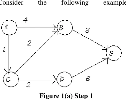
The above algorithm can be explained and understood better using an example. The example will briefly explain each step that is taken and how Dist is calculated. Consider the following example:
Figure 1(a) Step 1
The example is solved as follows:
Initial step
Dist[A]=0 ; the value to the source itself
Step 1
Adj[A]={B,C}; computing the value of the adjacent vertices of the graph
Dist[B]=4; Dist[C]=2;
Figure 1(b) Step 2
Figure: shortest path to vertices B, C from A
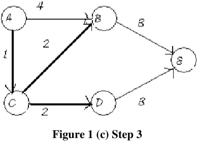
Step 2
Computation from vertex C
Adj[C] = {B, D};
Dist[B] > Dist[C]+ EdgeCost[C,B] 4 > 1+2 (True)
Therefore, Dist[B]=3;Dist[D]=2;
Figure 1 (c) Step 3
Figure: Shortest path from B, D using C as intermediate vertex
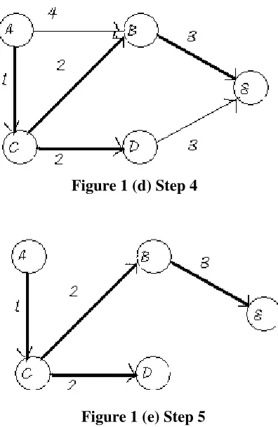
Dist[E]=Dist[B]+EdgeCost[B,E] =3+3=6;
Figure 1 (d) Step 4
Figure 1 (e) Step 5
Figure 1 Shortest Path using Dijkstra’s Algorithm
Adj[D]={E};
Dist[E]=Dist[D]+EdgeCost[D,E] =3+3=6
This is same as the initial value that was computed so Dist[E] value is not changed.
Step 3
And no more vertices, algorithm terminated. Hence the path which follows the algorithm is ACBE.
A* Algorithm: A* algorithm is a graph search algorithm that finds a path from a given initial node to a given goal node. It employs a "heuristic estimate" h(x) that gives an estimate of the best route that goes through that node. It visits the nodes in order of this heuristic estimate. It follows the approach of best first search. The secret to its success is that it combines the pieces of information that Dijkstra’s algorithm uses (favoring vertices that are close to the starting point) and information that Best-First-Search uses (favoring vertices that are close to the goal). In the standard terminology used when talking about A*, g(n)represents the exact cost of the path from the starting point to any vertex n, and h(n) represents the heuristic estimated cost from vertex n to the goal.
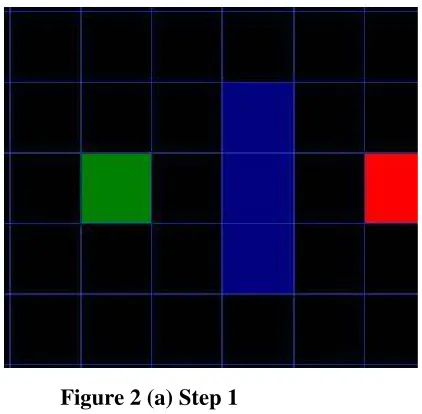
Let’s assume that we have someone who wants to get from point A to point B. Let’s assume that a wall separates the two points.
Figure 2 (a) Step 1
The map has a starting point, an ending point and some obstacles. Green is the starting point, Red is the ending point and Blue are the obstacles.
Step 1
We start by searching the 8 neighboring nodes of the Starting point.
Figure 2 (b) Step 2
Step 2
We calculate the Heuristics of those neighboring cells. F=G+H.
Figure 2 (c) Step 3
Step 3
Figure 2 (d) Step 4
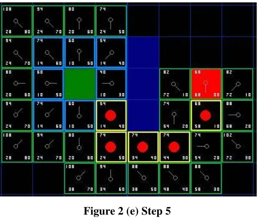
Final Result
The Red dots are the path that is chosen.
Figure 2 (e) Step 5
Figure 2 Shortest Path using A* Algorithm
heuristic is significant for theoretical analysis, it is not common to find such a heuristic in practice. Heuristics play a major role in search strategies because of exponential nature of the most problems. Heuristics help to reduce the number of alternatives from an exponential number to a polynomial number. Heuristic search has been widely used in both deterministic and probabilistic planning. Heuristic functions generally have different errors in different states. Heuristic functions play a crucial rule in optimal planning, and the theoretical limitations of algorithms using such functions are therefore of interest. Much work has focused on finding bounds on the behavior of heuristic search algorithms, using heuristics with specific attributes.
Comparison of A* and Dijkstra’s
Both the algorithms find the shortest distance between two nodes. Now, we would try to implement A star and Dijkstra’s on distributed system and compare them on running time and try and show that A star is a better than Dijkstra’s.
First of all let us cite the major differences between the two.
Note: Dijkstra’s Algorithm is special case of A* Algorithm, when h(n)=0.
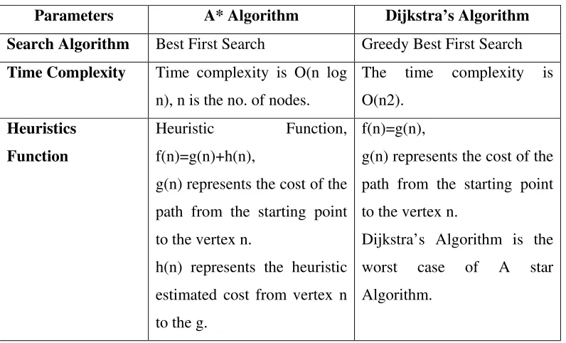
Parameters A* Algorithm Dijkstra’s Algorithm
Search Algorithm Best First Search Greedy Best First Search
Time Complexity Time complexity is O(n log n), n is the no. of nodes.
The time complexity is O(n2).
Heuristics
Function
Heuristic Function, f(n)=g(n)+h(n),
g(n) represents the cost of the path from the starting point to the vertex n.
h(n) represents the heuristic estimated cost from vertex n to the g.
f(n)=g(n),
g(n) represents the cost of the path from the starting point to the vertex n.
Dijkstra’s Algorithm is the worst case of A star Algorithm.
Table 1 Difference between A* Algorithm and Dijkstra’s Algorithm
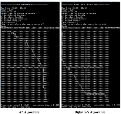
A* Algorithm Dijkstra’s Algorithm
Figure 3 Case 1 of Comparison between A* Algorithm and Dijkstra’s Algorithm
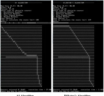
We are going to illustrate another example.
A* Algorithm Dijkstra’s Algorithm
Figure 4 Case 2 of Comparison between A* Algorithm and Dijkstra’s Algorithm
COMPARISION IN TIME (ms)
A* ALGORITHM DIJKSTRA’S ALGORITHM
CASE 1 67 CASE 1 146
COMPARISION IN PATH LENGTH (NODES)
A* ALGORITHM DIJKSTRA’S ALGORITHM
CASE 1 55 CASE 1 55
CASE 2 55 CASE 2 55
Table 2
As it can be seen, the lengths of paths do not vary in both the cases, but the time varies largely. This implies that, though both the algorithms provide the shortest path of equal lengths, the Dijkstra’s Algorithm scans more part of the map than the A* Algorithm does. Hence in these two cases and some others, A* Algorithm is better than the Dijkstra’s Algorithm.
Advantages and Disadvantages
A* is faster as compare to Dijkstra’s algorithm because it uses Best First Search whereas Dijkstra’s uses Greedy Best First Search.
Dijkstra’s is Simple as compare to A*.
The major disadvantage of Dijkstra’s algorithm is the fact that it does a blind search there by consuming a lot of time waste of necessary resources.
Another disadvantage is that it cannot handle negative edges. This leads to acyclic graphs and most often cannot obtain the right shortest path.
Dijkstra's algorithm has an order of n2 so it is efficient enough to use for relatively large problems.
Conclusion
Dijkstra's is essentially the same as A*, except there is no heuristic (H is always 0). Because it has no heuristic, it searches by expanding out equally in every direction, but A* scan the area only in the direction of destination. As you might imagine, because of this Dijkstra's usually ends up exploring a much larger area before the target is found. This generally makes it slower than A*. But both have their importance of its own, for example A* is mostly used when we know both the source and destination and Dijkstra’s is used when we don't know where our target destination is. Say you have a resource-gathering unit that needs to go get some resources of some kind. It may know where several resource areas are, but it wants to go to the closest one. Here, Dijkstra's is better than A* because we don't know which one is closest. Our only alternative is to repeatedly use A* to find the distance to each one, and then choose that path. There are probably countless similar situations where we know the kind of location we might be searching for, want to find the closest one, but not know where it is or which one might be closest. So, A* is better when we know both starting point and destination point. A* is both complete (finds a path if one exists) and optimal (always finds the shortest path) if you use an Admissible heuristic function. If your function is not admissible off - all bets are off.
REFERENCES
[1]Moshe Sniedovich, Dijkstra's Algorithm revisited, Department of Mathematics and Statistics ,The University of Melbourne, 2006
[3]Leo Willyanto Santoso, Alexander Setiawan, Andre K. Prajogo, Performance Analysis of Dijkstra and A*, Informatics Department, Faculty of Industrial Engineering, Petra Christian University, 2005
[4]Liang Dai, Fast Shortest Path Algorithm for Road Network and Implementation, Carleton University School of Computer Science, 2012 [5]Xiang Liu, Daoxiong Gong, A comparative study of Astar algorithms for
search and rescue in perfect maze, International Conference on Electric Information and Control Engineering, 2011
[6]Woo-Jin Seo, Seung-Ho Ok, Jin-Ho Ahn, Sungho Kang, Byungin Moon,
Study on the hazardous blocked synthetic value and the optimization
route of hazardous material transportation network based on A-star
algorithm, International Joint Conference on INC, IMS and IDC, 2012