Electrical percolation and the design of functional electromagnetic materials

(1)

Electrical percolation and the design of

functional electromagnetic materials

by

Ian J Youngs

A thesis submitted to the University of London for the Degree of

Doctor of Philosophy in Eiectrical Engineering

December 2001

Department of Eiectronic and Eiectrical Engineering

University Coilege London

Structures & Materials Centre

QinetiQ limited, Farnborough, Hants. G U I4 OLX.

(2)

ProQuest Number: U641968

INFORMATION TO ALL USERS

The quality of this reproduction is dependent upon the quality of the copy submitted.

In the unlikely event that the author did not send a complete manuscript and there are missing pages, these will be noted. Also, if material had to be removed,

a note will indicate the deletion.

uest.

ProQuest U641968

Published by ProQuest LLC(2015). Copyright of the Dissertation is held by the Author.

This work is protected against unauthorized copying under Title 17, United States Code. Microform Edition © ProQuest LLC.

ProQuest LLC

789 East Eisenhower Parkway P.O. Box 1346

(3)

Abstract

(4)

Declaration

Except where indicated otherwise in the acknowledgements section, the work contained in this thesis is the original research of the author and has not been previously submitted for a degree or comparable award of this or any other university or institution.

(5)

Acknowledgements

I would like to acknowledge the funding of this research primarily by Technology Group 04 of the MoD Corporate Research Programme, but also by Applied Research Package 04.

I wish to acknowledge the encouragement and support of my supervisors at UGL, Professors Hugh Griffiths and Alex Cullen (you have enabled me to fulfil my ambition); my many colleagues at QinetiQ:

- The management' Mike Pitkethly (thank you for giving me the opportunity), Steve Farmer and most recently Andy Treen, Alan Hooper for reviewing all my reports and papers and your ever constructive comments,

- For being there when I needed a sounding board and for providing me with hours from your projects: Chris Lawrence (one day I too may learn to love the plasmon), Steve Appleton, Steve Bleay, Andy Treen, Chris Gilmore, Eoin O’Keefe, John Cooper (now of DSTL), Nigel Comfort, Phil Roberts, John Smith (for advice on mathematical challenges) and Peter Lederer. Unfortunately, I hope this is just the start of electrical percolation at QinetiQ.

- For sharing the load on sample preparation and testing: Shahid Hussain (I hope you enjoy your PhD as much as I have enjoyed mine), Philip Drake (good luck in married life in Taiwan), Karl Lymer, Greg Fixter, Matt Bryanton, Paul Codling, Wendy Vine (thank you for inviting me to undertake the electromagnetic aspects of your Fellowship project, provision of quasicrystallline and nano aluminium powders and related micrographs, including the micrograph of carbon nanotubes), Uhbi Singh (for undertaking all other micrographs), Calvin Prentice (for preparing the carbon nanotubes), Alison Daniel, Sue Morris, Keith Park, Trevor Stickland, Tony Christopher (for particle density measurements), Alan Shakesheff (for particle size measurements) and my students Nick Jones and Sofy Fuchs.

Jed Marson and Gerhard Schaumburg of Novocontrol for opening my eyes to the potential of dielectric spectroscopy and training me in the use of the Novocontrol spectrometer; and Bob Clarke at NPL for advice on microwave measurements and uncertainty analysis.

I also thank my parents. Bill and Liz, for their encouragement and interest in my academic achievements throughout my education and career.

(6)

“substantia eluvies praebeo

f)

( WWW. arte-tv. com)

The concepts of percolation are applied in many fields of research, but the most vivid description of the phenomenon that I have discovered reads as follows

"... percolation is when you leave a wet sponge on a worktop and the water leaks out.”

(7)

List of tables

Table 2-1 : Summary of the principal effective media theories or models 56

Table 2-2: Percolation threshold occupation probabilities for various lattice types and for

both site and bond percolation [90, 91,157] 67

Table 2-3: Some critical exponents for the scaling laws [91,157] 70

Table 2-4: Summary of theoretical values for the exponents s and t, and for the limiting value of the dielectric loss tangent at the percolation threshold [91,157] 74 Table 2-5: Filling factors for some representative types of filler packing 76

Table 4-1 : Summary of physical properties of RTFE powders 162

Table 4-2: Summary of filler properties 164

Table 4-3: Summary of matrix:filler combinations investigated 164

Table 4-4: Filler loadings in microsphere:paraffin wax master batches 165

Table 4-5: Filler loadings in microsphere:epoxy master batches 165

Table 4-6: Filler loadings in carbon black:RTFE master batches 166

Table 4-7: Filler loadings in nano-aluminium:paraffin wax master batches 166 Table 4-8: Filler loadings in aluminium quasi-crystal:paraffin wax master batches 166

Table 4-9: Filler loadings in aluminium:paraffin wax master batches 167

Table 4-10: Filler loadings in carbon:paraffin wax master batches 167

Table 4-11 : Filler loadings in carbon:epoxy master batches 167

Table 4-12: Filler loadings in titanium diboride:RTFE master batches 168

Table 4-13: Filler loadings in nanotube:paraffin wax master batches 168

Table 4-14: Filler loadings of microsphere:paraffin wax test samples 169

Table 4-15: Filler loadings of microsphere:epoxy test samples 170

Table 4-16: Filler loadings of carbon black:RTFE test samples 171

Table 4-17: Filler loadings of nano-aluminium:paraffin wax test samples 172 Table 4-18: Filler loadings of aluminium quasi-crystal:paraffin wax test samples 173

Table 4-19: Filler loadings of aluminium:paraffin wax test samples 173

Table 4-20: Filler loadings of carbon:paraffin wax test samples 174

Table 4-21 : Filler loadings of carbon:epoxy test samples 174

Table 4-22: Filler loadings of titanium diboride:RTFE test samples 175

Table 4-23: Filler loadings of nanotube:paraffin wax test samples 175

Table 6-1 : Experimentally reported values for the percolation exponents (theory based on

spherical/circular particles) 209

Table 6-2: Fit parameter ranges and resolution for genetic algorithm 214

Table 6-3: Summary of testing the fitting performance of a two-pass genetic algorithm 218

Table 6-4: Fit parameters for carbon black:RTFE composites 227

Table 6-5: Summary of carbon black particle size analysis 229

(10)

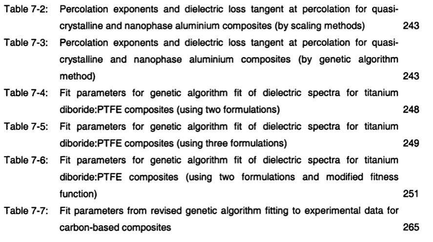
Table 7-2: Percolation exponents and dielectric loss tangent at percolation for quasi crystalline and nanophase aluminium composites (by scaling methods) 243 Table 7-3: Percolation exponents and dielectric loss tangent at percolation for quasi

crystalline and nanophase aluminium composites (by genetic algorithm

method) 243

Table 7-4: Fit parameters for genetic algorithm fit of dielectric spectra for titanium

diboride:PTFE composites (using two formulations) 248

Table 7-5: Fit parameters for genetic algorithm fit of dielectric spectra for titanium

diboride:PTFE composites (using three formulations) 249

Table 7-6: Fit parameters for genetic algorithm fit of dielectric spectra for titanium diboride:PTFE composites (using two formulations and modified fitness

function) 251

Table 7-7: Fit parameters from revised genetic algorithm fitting to experimental data for

(11)

List of figures

Figure 2-1 : Schematic representation of an electric dipole 30

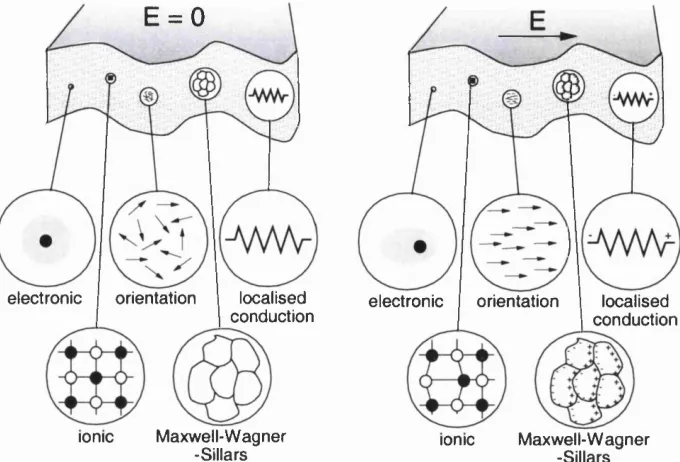
Figure 2-2: Schematic interpretation of polarisation processes 31

Figure 2-3: Clausius-Mossotti model for local field in a polarisable medium 33

Figure 2-4: The frequency response of electronic polarisability 36

Figure 2-5: The frequency response of orientation polarisability 39

Figure 2-6: Schematic of a two layer capacitor (a), its equivalent circuit (b), and an

equivalent single layer capacitor (c) 41

Figure 2-7: Charge hopping in a double potential well 44

Figure 2-8: Schematic frequency dependent dielectric response (excluding conduction) 48 Figure 2-9: Comparison of Debye-type models of the frequency dependent permittivity in

the complex plane 49

Figure 2-10: Schematic representation of an effective medium 53

Figure 2 - 1 1 : Conductivity as a function of filler volume fraction for an insulating matrix (with conductivity 1 x 10® S/cm) filled with spherical conducting particles (with conductivity 1 x 1 0 ® S/cm) with the filler particles occupying a simple cubic

lattice 78

Figure 2-12: Comparison of mixture conductivity as a function of filler volume fraction following the ‘geometric’ percolation models discussed in Section 2.5.3. (Calculations shown are for matrix and filler conductivities of 10'^® and 10® S/m, respectively; a matrix to filler particle size ratio of 100; filler particle radius of 1 0 pm; and square packing of the filler particles around the matrix

particles.) 83

Figure 2-13: Comparison of threshold volume fractions calculated by the ‘geometric’ percolation models discussed in Section 2.5.3 as a function of the matrix to filler particles size ratio. (Calculations shown are for the parameters used in

Figure 2-12, with the exception of the particle size ratio.) 83

Figure 2-14: Conductivity as a function of filler volume fraction for an insulating matrix (with conductivity 10'^ S/cm) filled with spherical conducting particles (with conductivity 10® S/cm) with the filler particles occupying a simple cubic lattice

(when relevant) 8 8

Figure 3-1 : Calculated frequency and filler fraction dependence of the complex permittivity for a conductor/insulator composite. Derived using the Maxwell-Garnett EMT, a matrix permittivity of 2.14, a filler conductivity of 1 S/m and assuming a

percolation threshold equal to unity 108

(12)

Figure 3-3: Calculated filler fraction dependence of the complex permittivity for a conductor/insulator composite at 1 GHz as a function of filler conductivity. Derived using the Maxwell-Garnett EMT, a matrix permittivity of 2.14 and

assuming a percolation threshold equal to unity. 1 1 0

Figure 3-4: Calculated frequency and filler fraction dependence of the complex permittivity for a conductor/insulator composite. Derived using the Bruggeman EMT, a matrix permittivity of 2.14, a filler conductivity of 1 S/m and assuming a

percolation threshold equal to V3. 1 1 1

Figure 3-5: Calculated frequency dependence of the complex permittivity for a conductor/insulator composite as a function of filler conductivity. Derived using the Bruggeman EMT, a matrix permittivity of 2.14, a normalised filler fraction of -0 . 0 1 and assuming a percolation threshold equal to V 3 . 1 1 2 Figure 3-6: Calculated filler fraction dependence of the complex permittivity for a

conductor/insulator composite at 1 GHz as a function of filler conductivity. Derived using the Bruggeman EMT, a matrix permittivity of 2.14 and assuming

a percolation threshold equal to V 3 . 1 13

Figure 3-7: Calculated frequency and filler fraction dependence of the complex permittivity for a conductor/insulator composite. Derived using the LIchtenecker EMT, a matrix permittivity of 2.14, a filler conductivity of 1 S/m and assuming a

percolation threshold equal to unity. 114

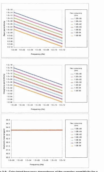
Figure 3-8: Calculated frequency dependence of the complex permittivity for a conductor/insulator composite as a function of filler conductivity. Derived using the LIchtenecker EMT, a matrix permittivity of 2.14, a normalised filler fraction of -0 . 0 1 and assuming a percolation threshold equal to unity. 1 15 Figure 3-9: Calculated filler fraction dependence of the complex permittivity for a

conductor/insulator composite at 1 GHz as a function of filler conductivity. Derived using the LIchtenecker EMT, a matrix permittivity of 2.14 and

assuming a percolation threshold equal to unity. 116

Figure 3-10: Calculated frequency and filler fraction dependence of the complex permittivity for a conductor/insulator composite. Derived using the McLachlan EMT, a matrix permittivity of 2.14, a filler conductivity of 1 S/m and assuming a

percolation threshold equal to V 3 . 117

Figure 3-11 : Calculated frequency dependence of the complex permittivity for a conductor/insulator composite as a function of filler conductivity. Derived using the McLachlan EMT, a matrix permittivity of 2.14, a normalised filler fraction of -0 . 0 1 and assuming a percolation threshold equal to V 3 . 118

Figure 3-12: Calculated filler fraction dependence of the complex permittivity for a conductor/insulator composite at 1 GHz as a function of filler conductivity. Derived using the McLachlan EMT, a matrix permittivity of 2.14 and assuming

(13)

Figure 3-13: Calculated frequency and filler fraction dependence of the complex permittivity for a conductor/insulator composite. Derived using the Doyle EMT (assuming all filler particles are contained in clusters for all filler fractions), a matrix permittivity of 2.14, a filler conductivity of 1 S/m and assuming a percolation

threshold equal to 0.212333. 120

Figure 3-14: Calculated frequency dependence of the complex permittivity for a conductor/insulator composite as a function of filler conductivity. Derived using the Doyle EMT (assuming all filler particles are contained in clusters for all filler fractions), a matrix permittivity of 2.14, a normalised filler fraction of -0.01 and assuming a percolation threshold equal to 0.212333. 121 Figure 3-15: Calculated filler fraction dependence of the complex permittivity for a

conductor/insulator composite at 1 GHz as a function of filler conductivity. Derived using the Doyle EMT (assuming all filler particles are contained in clusters for all filler fractions), a matrix permittivity of 2.14 and assuming a

percolation threshold equal to 0.212333. 122

Figure 3-16: Calculated frequency and filler fraction dependence of the complex permittivity for a conductor/insulator composite. Derived using the QCA-CP EMT, a matrix permittivity of 2.14, a filler conductivity of 1 S/m and assuming a

percolation threshold equal to %. 123

Figure 3-17: Calculated frequency dependence of the complex permittivity for a conductor/insulator composite as a function of filler conductivity. Derived using the QCA-CP EMT, a matrix permittivity of 2.14, a normalised filler fraction of -0.01 and assuming a percolation threshold equal to Va. 124 Figure 3-18: Calculated filler fraction dependence of the complex permittivity for a

conductor/insulator composite at 1 GHz as a function of filler conductivity. Derived using the QCA-CP EMT, a matrix permittivity of 2.14 and assuming a

percolation threshold equal to %. 125

Figure 3-19: Comparison of Havriliak-Negami fit to calculated Maxwell-Garnett data for composite with filler conductivity of 1 S/m and normalised filler fraction of -

0.0 1. 126

Figure 3-20: Havriliak-Negami fit (using two relaxation processes) to calculated Bruggeman

data for composite defined in Figure 3-19. 126

Figure 3-21 : Havriliak-Negami fit (using two relaxation processes and dc conductivity term) to calculated Bruggeman data for composite defined in Figure 3-19. 127 Figure 3-22: Havriliak-Negami fit (using three relaxation processes) to calculated

Bruggeman data for composite defined in Figure 3-19. 127

(14)

Negative values correspond to compositions below the percolation threshold.

Data is calculated using the Bruggeman EMT. 128

Figure 3-24: Dependence of the characteristic frequency, (o^, on filler conductivity and

distance from the percolation threshold (v-Vc). 128

Figure 3-25: Calculated frequency and filler fraction dependence of the complex permittivity for a conductor/insulator composite. Derived using Sheng’s EMT, a matrix permittivity of 2.14, a filler conductivity of 1 S/m and assuming a percolation

Figure 3-26: Calculated frequency dependence of the complex permittivity for a conductor/insulator composite as a function of filler conductivity. Derived using Sheng’s EMT, a matrix permittivity of 2.14, a normalised filler fraction of -0.01 and assuming a percolation threshold equal to 0.455071. 130 Figure 3-27: Calculated filler fraction dependence of the complex permittivity for a

conductor/insulator composite at 1 GHz as a function of filler conductivity. Derived using Sheng’s EMT, a matrix permittivity of 2.14 and assuming a

Figure 3-28: Calculated frequency and filler fraction dependence of the complex permittivity for a conductor/insulator composite. Derived using the Wakino EMT, a matrix permittivity of 2.14, a filler conductivity of 1 S/m and assuming a percolation

threshold equal to V3. 132

Figure 3-29: Calculated frequency dependence of the complex permittivity for a composite as a function of filler conductivity. Derived using the Wakino EMT, a matrix permittivity of 2.14, a normalised filler fraction of -0.01 and assuming a

percolation threshold equal to V 3 . 133

Figure 3-30: Calculated filler fraction dependence of the complex permittivity for a composite at 1 GHz as a function of filler conductivity. Derived using the Wakino EMT, a matrix permittivity of 2.14 and assuming a percolation

threshold equal to V 3 . 134

Figure 3-31 : Variation of lower characteristic frequency, with filler fraction. (Values from the fit equation are used to demonstrate consistency with statistical percolation theory, which predicts values for the slope and intercept equal to 2.63 and 10.72, respectively. Data is taken from Figure 3-10.) 135 Figure 3-32: Variation of the upper characteristic frequency, At, with filler conductivity.

(Values from the fit equation are used to demonstrate consistency with the MWS relaxation frequency, which predicts values for the slope and intercept equal to 1.00 and -0.54, respectively. Data is taken from Figure 3-10.) 135 Figure 3-33: Calculated filler fraction dependence of the complex permittivity for a

composite at 1 GHz and with a filler conductivity of 10® S/m as a function of the percolation threshoid. Derived using the McLachlan EMT, a matrix

(15)

Figure 3-34; Calculated filler fraction dependence of the complex permittivity for a composite at 1 GHz and with a filler conductivity of 10® S/m as a function of the ratio s:t (keeping t constant and equal to unity). Derived using the McLachlan EMT, a matrix permittivity of 2.14 and assuming a percolation

threshold equal to V3. 137

Figure 3-35: Calculated filler fraction dependence of the complex permittivity for a composite at 1 GHz and with a filler conductivity of 10® S/m as a function of the ratio s:t (keeping s constant and equal to unity). Derived using the McLachlan EMT, a matrix permittivity of 2.14 and assuming a percolation

Figure 3-36: Calculated frequency dependence of the complex permittivity for a composite with a filler conductivity of 10 S/m and normalised filler fraction of -0.01 as a function of the percolation threshold. Derived using the McLachlan EMT, a

matrix permittivity of 2.14 and assuming s=0.73 and t=1.9. 139

Figure 3-37: Calculated frequency dependence of the complex permittivity for a composite with a filler conductivity of 10 S/m as a function of the ratio s:t (keeping t constant and equal to unity). Derived using the McLachlan EMT, a matrix permittivity of 2.14 and assuming a percolation threshold equal to V 3 . 140

Figure 3-38: Calculated frequency dependence of the complex permittivity for a conductor/insulator composite with a filler conductivity of 10 S/m as a function of the ratio s:t (keeping s constant and equal to unity). Derived using the McLachlan EMT, a matrix permittivity of 2.14 and assuming a percolation

Figure 3-39: Filler fraction in clusters (top) and fill fraction of clusters in medium (bottom) as a function of total filler fraction for various functions representing the

distribution of filler particles in Doyle’s EMT. 142

Figure 3-40: Calculated frequency and filler fraction dependence of the complex permittivity for a conductor/insulator composite. Derived using the Doyle EMT (with Sheng’s model for the proportion of filler particles forming clusters), a matrix permittivity of 2.14, a filler conductivity of 1 S/m and assuming a percolation

Figure 3-41 : Calculated frequency dependence of the complex permittivity for a conductor/insulator composite as a function of filler conductivity. Derived using the Doyle EMT (with Sheng’s model for the proportion of filler particles forming clusters), a matrix permittivity of 2.14, a normalised filler fraction of -0.01 and assuming a percolation threshold equal to 0.339645. 144 Figure 3-42: Calculated filler fraction dependence of the complex permittivity for a

(16)

particles forming clusters), a matrix permittivity of 2.14 and assuming a

Figure 3-43: Calculated frequency dependence of the complex permittivity for a conductor/insulator composite as a function of filler particle radius. Derived using the QCA-CP EMT, a matrix permittivity of 2.14, a filler conductivity of 10' ^ S/m, a normalised filler fraction of -0.01 and assuming a percolation

threshold equal to %. 146

Figure 3-44: Calculated filler fraction dependence of the complex permittivity for a conductor/insulator composite at 10 GHz as a function of filler particle radius. Derived using the QCA-CP EMT, a matrix permittivity of 2.14, a filler conductivity of 10"^ S/m and assuming a percolation threshold equal to 14. 147 Figure 3-45: Calculated filler fraction dependence of the complex permittivity for a

conductor/insulator composite at 10 GHz as a function of filler particle radius. Derived using the QCA-CP EMT, a matrix permittivity of 2.14, a filler conductivity of 1 S/m and assuming a percolation threshold equal to 14. 148 Figure 3-46: Calculated frequency dependence of the complex permittivity for a

conductor/insulator composite as a function of filler aspect ratio for oblate spheroidal particles. Derived using the MG EMT, a matrix permittivity of 2.14, a filler conductivity of 1 S/m, a normalised filler fraction of -0.01 and assuming

a percolation threshold equal to unity. 149

Figure 3-47: Calculated frequency dependence of the complex permittivity for a conductor/insulator composite as a function of filler aspect ratio for prolate spheroidal particles. Derived using the MG EMT, a matrix permittivity of 2.14, a filler conductivity of 1 S/m, a normalised filler fraction of -0.01 and assuming

a percolation threshold equal to unity. 150

Figure 3-48: Calculated filler fraction dependence of the complex permittivity for a conductor/insulator composite at 1 GHz as a function of filler aspect ratio for oblate spheroidal particles. Derived using the MG EMT, a matrix permittivity of 2.14, a filler conductivity of 1 S/m, and assuming a percolation threshold

equal to unity. 151

Figure 3-49: Calculated filler fraction dependence of the complex permittivity for a conductor/insulator composite at 1 GHz as a function of filler aspect ratio for prolate spheroidal particles. Derived using the MG EMT, a matrix permittivity of 2.14, a filler conductivity of 1 S/m, and assuming a percolation threshold

equal to unity. 152

Figure 3-50: Calculated frequency and filler fraction dependence of the complex permittivity for a conductor/insulator composite. Derived using the Lagarkov-Sarychev low frequency EMT, a matrix permittivity of 2.14, a filler conductivity of 10^ S/m, a particle aspect ratio of 100 and assuming a percolation threshold equal

(17)

Figure 3-51 ; Calculated frequency dependence of the complex permittivity for a conductor/insulator composite as a function of filler conductivity. Derived using the Lagarkov-Sarychev low frequency EMT, a matrix permittivity of 2.14, a particle aspect ratio of 1 0 0, a normalised filler fraction of -0 . 0 1 and

assuming a percolation threshold equal to 0.0414747. 154

Figure 3-52: Calculated filler fraction dependence of the complex permittivity for a conductor/insulator composite at 1 GHz as a function of filler conductivity. Derived using the Lagarkov-Sarychev low frequency EMT, a matrix permittivity of 2.14, a particle aspect ratio of 100 and assuming a percolation threshold

equal to 0.0414747. 155

Figure 3-53: Calculated frequency dependence of the complex permittivity for a conductor/insulator composite as a function of shell thickness of core-shell particles with a conducting shell and an air-filled core. Derived using the Sihvola-Lindell EMT, a matrix permittivity of 2.14, a shell conductivity of 1 S/m, a normalised filler fraction of -0 . 0 1 and assuming a percolation threshold equal

to unity. 156

Figure 3-54: Calculated shell thickness dependence of the normalised complex permittivity for a composite as a function of fiiler fraction at the frequency of maximum ioss for a solid particle. Normalisation is with respect to the properties for the solid particle at each filler fraction. Derived using the Sihvola-Lindell EMT, a matrix permittivity of 2.14, a shell conductivity of 1 S/m, and assuming a

percolation threshold equal to unity. 157

Figure 3-55: As Figure 3-54, but the permittivity of the coating is taken to be fully complex with a real component equal to 10. (All previous data has assumed a purely

imaginary permittivity for the conductive phase). 158

Figure 3-56: Comparison of static permittivity predicted by the effective medium and percolation models analysed in Chapter 3. The results are plotted against the percolation threshold predicted by each model. Values relate to composites with a matrix permittivity of 2.14, a filler conductivity of 0.01 S/m and a normalised filler fraction of -0.01. The lower graph shows an expanded area

of the upper graph. 159

Figure 3-57: Comparison of MWS relaxation frequencies predicted by the effective medium and percolation models analysed in Chapter 3. The results are plotted against the percolation threshold predicted by each model. Values relate to composites with a matrix permittivity of 2.14, a filler conductivity of 0.01 S/m and a normalised filler fraction of -0.01. The lower graph shows an expanded

area of the upper graph. 160

(18)

data presented relates to a conductor-insulator composite with a matrix

permittivity of 2.14 and a filler conductivity of 10® S/m. 161

Figure 3-59: Comparison of the filler fraction dependence of the ac conductivity at 1 GHz for the effective medium and percolation models analysed in Chapter 3. The data presented relates to a conductor-insulator composite with a matrix

permittivity of 2.14 and a filler conductivity of 1 S/m 161

Figure 4-1 : Particle size distributions of RIFE powders 163

Figure 4-2: Schematic of Novocontrol low and Intermediate frequency dielectric

measurement system. 176

Figure 4-3: Schematic of BDS2100 RF sample cell 178

Figure 4-4: Schematic of the high frequency measurement system. 180

Figure 4-5: Schematic of 7mm coaxial sample cell and airgap dimensions (D„) 180 Figure 4-6: Polar diagram representation of circle of uncertainty approach for determining

phase uncertainty 183

Figure 5-1 : Frequency dependence of the complex permittivity (real part with solid symbols, imaginary part with open symbols) for a selection of silver coated

microsphere:paraffln wax formulations 185

Figure 5-2: The effectiveness of the correction to low frequency measurements using the results for the 5% microsphere:paraffin wax system as an example 187 Figure 5-3: Permittivity spectra for silver coated microsphere:paraffln wax formulations

below the percolation threshold 189

Figure 5-4: Permittivity spectra for silver coated microsphere:paraffin wax formulations

above the percolation threshold 189

Figure 5-5: Backscatter SEM image of 5 vol% microsphere:paraffin wax (XC00718) showing a section through the thickness of a die pressed sample 191 Figure 5-6: Backscatter SEM image of 15 vol% microsphere:paraffin wax (XC00723)

showing a section through the thickness of a die pressed sample 191 Figure 5-7: Backscatter SEM image of 30 vol% microsphere:paraffin wax (XC00729)

showing a section through the thickness of a die pressed sample 191 Figure 5-8: SEM image of a broken microsphere within a die pressed microsphere:paraffin

wax sample 191

Figure 5-9: Filler fraction dependence of the real permittivity for microsphere:paraffin wax formulations based on master batch quantities compared to Effective Medium

Theories (EMTs) 192

Figure 5-10: Filler fraction dependence of the imaginary permittivity for microsphere:paraffin wax formulations based on master batch quantities

compared to Effective Medium Theories (EMTs) 192

Figure 5-11 : Filler fraction dependence of the conductivity (at 1 Hz) for microsphere:paraffin wax formulations based on master batch densities

(19)

Figure 5-12: Determination of the critical percolation exponents, s and t, for the conductivity and real permittivity from the experimental data near the percolation threshold 194 Figure 5-13: Comparison of the measured frequency dependence of the dielectric loss

tangent with that predicted by a 3-D resistor-capacitor model 195

Figure 5-14: High frequency permittivity spectra of selected microsphere:paraffin wax

composites showing slopes of traces between 0.5 and 3 GHz 197

Figure 5-15: Temperature dependence of the ac conductivity (at 113 MHz) for 15, 16 and

30 % filler fractions 198

Figure 5-16: Data of Figure 5-15 plotted for comparison to the Austin-Mott Variable Range

Hopping model 198

Figure 5-17: Data of Figure 5-15 plotted for comparison to the Austin-Mott Activated

Poiaron Hopping model 199

Figure 5-18: Frequency dependence of the complex permeability for selected silver coated

microsphere:paraffin wax formulations 199

Figure 5-19: Comparison of measured complex permeability for 30% filler fraction with theoretical prediction based on equation (2-115) for eddy currents in a

conducting slab 2 0 0

Figure 5-20: Comparison of measured complex permeability for 5, 15 and 30% filler fractions with theoretical prediction based on equation (2-115) for eddy

currents in a conducting sphere 2 0 0

Figure 5-21: Calculated complex permeability for filler fractions of 5,15 and 30% based on

Mie theory 201

Figure 5-22: Comparison of mean microsphere radius and silver coating thickness to skin

depth for a conductivity of 5x10^ S/m 201

Figure 5-23: Permittivity spectra for silver coated microsphere:epoxy formulations 203 Figure 5-24: Fit of Debye response to permittivity spectra for 15 vol% microsphere:epoxy

formulation (Fit parameters: 1=4.78x10®, Ae=4.39, 6o,=4.95, a=0.264, p=1,

Odc=7.38x10'^) 204

Figure 5-25: Fit of two Dissado-Hill relaxation processes to permittivity spectra for 15 vol% microsphere:epoxy formuiation (Fit parameters: xi=3.09x10'®, Aei=0.57, e«i=3.0, ni=0.83, mi=0.629; 12=2.83x10'^°, Aei=3.01, e«,i=2.5, ni=0.639,

mi=0.118) 204

Figure 5-26: Filler fraction dependence of the complex permittivity for microsphere:epoxy formulations based on master batch quantities compared to Effective Medium

Theories 205

Figure 5-27: Scanning electron micrographs of microsphere:epoxy test samples with nominal fill fractions of 0.1 (top left), 0.2 (top right), 0.3 (bottom left) and 0.4

(bottom right) 206

Figure 6-1 : Flow chart representation of basic genetic algorithm 211

(20)

Figure 6-3: Demonstration of convergence of genetic algorithm towards optimum solution

(legend shows generation number) 215

Figure 6-4: Convergence of algorithm for multiple independent runs (Population size = 50,

Pcross — 0.7, Pmut^0.05) 216

Figure 6-5: Comparison of fit spectra to test spectra after 20 generations

(Population size = 50, Pcross = 0.7, Pmu«=0.05) 216

Figure 6-6: Accuracy of fit for a filler conductivity of 1 S/m 219

Figure 6-7: Accuracy of fit for a filler conductivity of 10^ S/m 219

Figure 6-8: Accuracy of fit for a filler conductivity of 10^ S/m 219

Figure 6-9: Results of fitting for Of =1 S/m and Vi<Vc<V2 (Vi = 0.175 blue, V2 = 0.225 red) 220 Figure 6-10: Results of fitting for Of=1 S/m and V2<Vi<Vc (Vi = 0.175 blue, V2 = 0.125 red) 220 Figure 6-11 : Results of fitting for Of =1 S/m and Vc<Vi<V2 (Vi = 0.225 blue, V2 = 0.275 red) 220 Figure 6-12: Results of fitting for Of =10^ S/m and Vi<Vc<V2 (Vi =0.175 blue, V2 =0.225 red) 221 Figure 6-13: Results of fitting for o, =10’^ S/m and Vi<Vc<V2 (Vi=0.175 blue, V2=0.225 red) 221 Figure 6-14: Influence of reproduction probabilities on fitness for test data spanning the

percolation threshold and a filler conductivity of 1 S/m 2 2 2

Figure 6-15: Influence of number of generations used in each pass on fitness for test data spanning the percolation threshold and a filler conductivity of 1 S/m 222 Figure 6-16: Results of fitting as for Figure 6-9 but with 40 generations used in 1** pass 223 Figure 6-17: Experimental dielectric spectra for carbon black:PTFE formulations 224 Figure 6-18: Variation of permittivity with PTFE particle size at 1 GHz for carbon

black:PTFE formulations (for nominal filler fractions of 1 and 10%) 225 Figure 6-19: Comparison of genetic algorithm fit to experimental dielectric spectra of

carbon black:PTFE composites 226

Figure 6-20: Comparison of experimentally determined percolation thresholds for

carbon black:PTFE composites to geometric percolation models 228

Figure 6-21 : SEM images of free carbon black particles 228

Figure 6-22: SEM images of 55 pm PTFE-based composites containing

1 vol% (left) and 10 vol% (right) carbon black 229

Figure 6-23: Comparison of experimentally determined percolation thresholds for carbon black:PTFE composites to a geometric percolation model incorporating ellipsoidal matrix particles and using an aspect ratio of 0.1 231

Figure 7-1 : Dielectric spectra of aluminium:paraffin wax composites 239

Figure 7-2: Dielectric spectra of nanophase aluminium:paraffin wax composites 239 Figure 7-3: Dielectric spectra of aluminium quasi-crystals:paraffin wax composites 239 Figure 7-4: Filler fraction dependence of dielectric properties at 1 GHz for composites filled

with the three types of aluminium-based particles. Comparison of data taken using the radio-frequency (RF) and microwave (MW) measurement systems. 240 Figure 7-5: SEM images of composites loaded with approximately 10% quasicrystalline

(21)

Figure 7-6: Filler fraction dependence properties of conductivity at 1 Hz for composites

filled with the three types of aluminium-based particles. 242

Figure 7-7: Determination of critical percolation exponent s for quasicrystalline and

nanophase aluminium filled paraffin wax composites 242

Figure 7-8: Electromagnetic response of a thin (compared to the wavelength) layer of

composite at its respective percolation threshold 245

Figure 7-9: Electromagnetic response of a layer (quarterwave thick at 100 MHz) of

composite at its respective percolation threshold 245

Figure 7-10: Electromagnetic response of 0.263 m thick layers of composite at their

respective percolation threshold 245

Figure 7-11 : Dielectric spectra for titanium diboride:PTFE composites 248

Figure 7-12: Comparison of genetic algorithm fit to dielectric spectra for titanium

diboride:PTFE composites (using two formulations) 248

Figure 7-13: Comparison of genetic algorithm fit to dielectric spectra for titanium

diboride:PTFE composites (using three formulations) 249

Figure 7-14: Comparison of genetic algorithm fit using two formulations to dielectric spectra for titanium diboride:PTFE composites in loss tangent and conductivity

formats 250

Figure 7-15: Comparison of genetic algorithm fit to dielectric spectra for titanium diboride:PTFE composites (using two formulations and modified fitness

function) 250

Figure 7-16: Comparison of measured filler fraction dependence of dielectric properties for titanium diboride:PTFE composites with results predicted using fit parameters 252 Figure 7-17: Comparison of measured filler fraction dependence of dielectric properties for

titanium diboride:PTFE composites with results predicted using effective

medium and percolation models analysed in Chapter 3 252

Figure 7-18: Measured magnetic permeability spectra for titanium diboride:PTFE

composites 253

Figure 7-19: Comparison of measured permeability spectra for titanium diboride:PTFE composites to spectra predicted by Mie theory with a filler conductivity of

3x10^ S/m (from genetic algorithm prediction) 253

Figure 7-20: Comparison of measured permeability spectra for titanium diboride: PTFE composites to spectra predicted by Mie theory with a filler conductivity of

1x10® S/m 254

Figure 7-21 : Schematic representations of the allotropes of carbon [232] 255

Figure 7-22: TEM image of carbon nanotubes 257

Figure 7-23: Dielectric spectra of graphite:paraffin wax composites 259

Figure 7-24: Dielectric spectra for buckytube:paraffin wax composites 259

(22)

Figure 7-26: Comparison of dielectric spectra for carbon and microsphere filled composites

at filler fractions closest to 1 0 vol% 260

Figure 7-27: Comparison of genetic algorithm fit using McLachlan’s GEM to experimental

data for graphite:paraffin wax system 261

data for graphite:epoxy resin system 261

data for buckytube:paraffin wax system 262

Figure 7-30: Comparison of revised genetic algorithm fit using McLachlan’s GEM to

experimental data for the graphite:paraffin wax system 263

Figure 7-31 : Comparison of revised genetic algorithm fit using McLachlan’s GEM to

experimental data for the graphite:epoxy resin system 264

(23)

Glossary

ac ar b B BDS c CP Co d dc c/

d m , I

e E Eay Ef El Elo EMT f f(z) he fm axtanS FRA particle radius, fibre half length

mantissa of a reai number, maximum packing fraction in an agglomerate,

aspect ratio area, surface area a function of aspect ratio, shape factor

alternating current aspect ratio slab thickness, fibre radius,

sample inner diameter magnetic induction

Broadband Dielectric Spectrometer speed of light,

volume fraction of crystal phase in the matrix,

sample outer diameter capacitance,

a constant representing the rate of evolution of the universal interfacial energy

Coherent Potential

capacitance of empty capacitor distance, thickness, dimension, ratio of filler plus adsorbed matrix volume to base filler volume, capacitor plate separation electric displacement field, diffusion coefficient, diameter of capacitor,

network analyser effective directivity average electric displacement direct current

fractal dimension

matrix and filler particle diameter electronic charge,

ellipticity electric field average electric field Fermi energy local electric field local field at time zero effective medium theory frequency

scaling function

eddy current permeability multiplier frequency of maximum loss factor frequency of maximum loss tangent Frequency Response Analyser frequency of maximum loss in electric

modulus spectra (relaxation frequency)

f / frequency of maximum loss in

permittivity spectra (relaxation frequency)

F force

F(z) finite size scaling function

F±(Xi) scaling functions atx)ve (+) and below (-) the percolation threshold

Fr restoring force

G conductance

GEM General Effective Medium

g(r) probability that two sites are connected by a distance r

depolarisation factors for rods G* interfacial excess energy

h sample height

H magnetic field

h, A Planck’s constant

/■ current

I network analyser isolation

j V-1

J current density

k force constant, wave vector, uncertainty coverage factor km,k Wave vector in component material Ko interfacial energy at time zero

ke Boltzmann constant

I length of (rod-like) filler particle

L side length of tx)und space,

depolarisation factor, sample length,

network analyser linearity

LF low frequency

hoc localisation length

m coefficient in Dissado-Hill model, coefficient in Lynch formula

M electric modulus,

network analyser effective test port match

m. mass of anion

m+ mass of cation

M '(0) initial net change in dipole moment on application of electric field

nte electron mass

mgff effective mass

Mk kth moment of the cluster size distribution

mm.f mass of matrix and filler

m„ nuclear mass

Mtm network analyser mismatch

MW microwave

MWCN Multi-walled cartx>n nanotubes

(24)

N n(E) n(Ef) No nph NRW n, P P

P c m a s P .

P h c p ,P ' Pi

P ic

Pmul

P o P u m Pr,t,a

PTCR PTFE

P to ta l

q QC OCA r R R. a RF R fm,f

integer number of charges,

number of charges yet to experience a collision,

exponent of temperature dependence in Sheng’s tunneiiing model, ionic concentration,

coefficient in Dissado-Hill model, population size

number of dipoles per unit volume, number of unit cells, number of particles,

size of sub-population density of states

density of states at the Fermi level number of dipoles at time zero number of phonons

Nicolson-Ross-Weir

number of clusters of size s - the cluster number

electric dipole moment, protiability of site occupation electric polarisation,

fraction of sites in the infinite cluster, probability that the outermost layer of filler particles covering a matrix particle has percolated

critical site occupation probability (also with superscript bond or site indicating type of percolation)

crossover probability electronic polarisation hopping probability ionic polarisation

polarisation due to localised conduction mutation probability

orientation polarisation

Maxwell-Wagner-Sillars polarisation reflected, transmitted, absorbed power Postive Temperature Coefficient of Resistance

Polytetrafluoroethylene total polarisation Charge Quasicrystalline

Quasicrystalline Approximation distance, radius

Atomic radius, ionic radius, resistance,

transition probability, reflection coefficient,

residual uncertainty from combined random effects in network analyser measurements

anion radius cation radius Radio Frequency transition rate

radius of matrix and filler particles

S SEM to tend tanÔEc TEM u U,*nm Us V V V' Va.b

Vcp Vi, II

V m .t V m a a te r batch Vaam pte Va(p) w Vf Vio W o Xo y Y

Y i,m ,f Z

average radius of clusters of size s exponent of frequency dependence of ac conductivity,

percolation exponent for permittivity, cluster size

average cluster size

scanning electron microscopy (n,m = 1,2) scattering parameters from a two port device

time,

percolation exponent for conductivity, thickness of capacitor plates, layer thickness

temperature,

network analyser tracking

time at which observation of system starts

(dielectric) ioss tangent

magnetic loss tangent due to eddy currents

Transmission Electron Micrograph dummy variable in Kramers-Kronig relationships

uncertainty in S-parameter phase uncertainty in S-parameter magnitude particle volume

volume, voltage, filler volume fraction normalised filler fraction

lower and upper critical volume fractions for conductivity critical filler volume fraction, percolation threshold close-packing filler fraction

volume fractions for regions of type I and II

matrix and filler volume fraction filler fraction in master batch filler fraction in test sample

ratio of cluster number at p to cluster number at pc

Energy

energy with no applied electric field activation energy

band gap energy distance,

percolation exponent for frequency dependence of conductivity, number of layers of filler particles covering a matric particle critical fraction of matrix particle surface covered by filler particles displacement at time zero percolation exponent for frequency dependence of permittivity Admittance

component admittance collision frequency,

(25)

z z z, Zempiy Zl Z o Z . a CXl,2 Oe Ot CCI CCo P

Ya b

Ye Y Ym,f 5 Se c Ae A a ^i*r) c max

Sa Ccorraclad Cmtf Cmaaaurad Bo Br fr-Brti

dependence of the loss tangent atomic number

number of charges on anion number of charges on cation impedance of empty sample cell load impedance

characteristic impedance of a transmission line

sample impedance electric polarisability, coefficient in Havriliak-Negami representation of complex permittivity, percolation exponent,

probability of a contact forming between neighbouring sites structural crossover concentrations electronic polarisability

polarisability of filler particle ionic polarisability

orientation polarisability coefficient in Havriliak-Negami representation of complex permittivity, reciprocal skin depth

percolation exponent bond restoration constant, percolation exponent core volumes

damping factor in electronic polarisation

damping factor in ionic poiarisation surface tension of matrix and filler particles

(loss) phase angle

phase angle for eddy currents difference between filler and matrix permittivity,

dielectric relaxation amplitude difference between filler and matrix conductivity

absolute dielectric constant or permittivity,

effective permittivity of a mixture upper, lower bounds for permittivity maximum imaginary permittivity permittivity of arbitrary reference material

arbitrary permittivity airgap corrected permittivity permittivity of matrix and filler components

measured permittivity free space permittivity Relative permittivity

high frequency limit of permittivity, relative permittivity above a relaxation process

low frequency limit of permittivity, relative permittivity below a relaxation process

Ç characteristic frequency marking the transition between classical and quantum mechanical effects

r\ matrix viscosity,

characteristic impedance

e time interval

6b Debye temperature

A a chain length factor,

wavelength keft effective wavelength

ko free space wavelength

H electron mobility,

absolute magnetic permeability, chemical potential

fCcorraaad airgap corrected permeability fif filler permeability

fimaaaurad measured permeability permeability of free-space fip permeability of a particle

relative magnetic permeability

V velocity of sound,

percolation exponent

Vph phonon frequency

Va specific void space

^ correlation length

p density of composite,

reflection coefficient Pm,! density of matrix and filler

a conductivity,

percolation exponent cr*, ac conductivity

aa cluster conductivity

<7* dc conductivity a,n effective conductivity ai,m,i component conductivity

r relaxation time,

Fisher percolation exponent, time beyond which electron propagation becomes diffusive, transmission coefficient

0 filling factor

X absolute electric susceptibility

Xo low frequency limit of susceptibility

X , relative electric susceptibility

(o angular frequency

(ÛI (lower) characteristic frequency (Og fraction of filler phase in the infinite

cluster

oimis MWS relaxation frequency

(ÛO resonant frequency,

(upper) characteristic frequency o)p frequency of peak dielectric loss,

(upper) characteristic frequency

(26)

Introduction

1.1 Definition

It is Important to define, from the outset, the scope of the title - 'Electrical percolation and the design of functional electromagnetic materials”

The phrase “functional electromagnetic materials” is used here to describe any material consisting of more than one component and where the combination of materials is chosen specifically to achieve a desired response to an incident electromagnetic wave. In this sense each component is assumed to possess a unique combination of permittivity and permeability, which together define the refractive index and impedance of a material. The composite material is therefore heterogeneous, although the heterogeneity may be at any dimensional scale smaller than the physical dimensions of the test piece. This includes heterogeneities at the molecular level, as represented by interpenetrating networks of different polymers. The study is further constrained by considering such materials where they are isotropic on a scale comparable to the incident wavelength. This is the so-called quasi-static limit. Thus, the electromagnetic properties of the composite can be expected to be a function of the relative proportions of the constituents.

A key feature of an electromagnetic wave is the frequency of the sinusoidal oscillations of the electric (and magnetic) field components of the wave. This frequency defines the nature of the microscopic mechanisms within a material that determine the macroscopic electromagnetic response of the bulk material. It follows that the frequency dependence of a material's permittivity (and permeability) is vital to the identification of the prevailing mechanism(s) and the subsequent optimisation of a material's formulation to achieve a desirable electromagnetic response for a particular application. For the purpose of this study the frequency range is restricted to frequencies below 100 GHz, with primary focus on the radio and microwave ranges, between 1 kHz and 20 GHz. Typical applications require materials for electromagnetic shielding or materials to simulate the dielectric response of human tissue.

(27)

1.2 Objective

The objective of this study is to establish design guidelines capable of specifying composite material formulations that could reliably and reproducibly yield improved electromagnetic performance through utilisation of critical behaviour near the percolation threshold. This will be achieved by identifying the most appropriate and possibly improved theoretical model for the electromagnetic properties of composite material systems consisting of conducting particles dispersed in an insulating matrix. The model should be accurate over the maximum achievable range of filler volume loading and frequency. However, most emphasis will be focused on accurately modelling the properties of highly interacting systems (i.e. where the conducting particles approach close contact, near the percolation threshold). Experimental studies will be used to validate the theory.

1.3 Background

The study of the electromagnetic properties of composite materials is far from just academic curiosity. The design of materials with specific dielectric (including conduction) and magnetic properties is central to meeting applications in the communication, construction, defence, food, medical, power and transport markets. Applications typical of these markets include: electromagnetically shielded enclosures for equipment and base-stations; in-process quality control and cure monitoring in fibre-reinforced plastic manufacture; camouflage materials and remote sensing; simulants for microwave heating; microwave imaging of tissue; geophysical surveying and flow monitoring in pipelines; and in-situ smart sensing for health monitoring in aircraft and bridges.

Similarly wide ranges of material types are employed, both as fillers and host matrices. Probably the most significant class of host matrices are insulating polymers. These can include: thermoplastics (for example polyethylene, polypropylene, polytetrafluoroethylene, etc) which can be in different physical forms such as essentially fully dense solids or foams and can possess varying degrees of crystallinity or be entirely amorphous; thermosets (for example epoxies, vinyl esters and urethanes) which can be chosen to exhibit varying degrees of elasticity depending on their glass transition temperature. Hybrids of these systems, in the form of copolymers and blends, are also widely available for more specific applications. An alternate class of host matrix are the insulator ceramics (such as alumina or zirconia) for applications where higher dielectric strength or higher temperature operation is required.

(28)

ceramics including titania and the alkali earth metal titanates, piezoelectrics, liquid crystals or superconductors. Magnetic properties can also be imparted using transition metal elements (e.g. iron, nickel and cobalt) or ferromagnetic ceramics (e.g. barium hexaferrite); alternatively metallised particulates that can sustain current loops may be of use.

The use of composite materials provides greater degrees of freedom for the electromagnetic engineer to achieve a specific performance target than are available from any of the individual components. In addition, there is scope to take advantage of effects that only occur in the multi- component system. An example might be the absorption generated by the combination of a conductive filler in an insulating matrix, due to the Maxwell-Wagner effect, which is not present in either of the constituent materials in their bulk forms. Moreover, the use of composite materials are essential in today’s high-tech environment where applications require a diverse range of mechanical, electrical and chemical properties, often to fulfil a multi-functional role. For example, a filler could be chosen to impart dielectric properties to the composite whilst the matrix is chosen to provide impact performance or tensile strength. In such a case, the composite is of more practical value than either of the components.

1.4 Overview

This thesis is organised in the following manner. It commences with a review and discussion of the relevant literature. The review addresses the frequency, temperature and filler fraction dependencies of the electromagnetic response of materials. It embodies a discussion of effective media and percolation theories, including the nature of critical behaviour near the percolation threshold. These elements are contained in Chapter 2. A more detailed theoretical analysis of effective medium and percolation theories can be found in Chapter 3. This is provided to aid interpretation of the experimental data and to identify design rules for optimising and improving the performance of conductor-insulator composites with particular relevance to shielding applications. Discussion of the literature is also used to shape the experimental strategy of the study, which is recorded in Chapter 4 together with descriptions of the experimental techniques employed. Chapter 5 presents the experimental results and discussion of a pseudo-model system based on silver-coated microspheres. The proposed new genetic algorithm based method for analysing experimental data is described in Chapter 6, which concludes with a discussion of the implications for an improved design process for electromagnetically-functional composite materials. Chapter 7 presents and discusses the results for a range of other conductive filler materials. Finally, conclusions and recommendations are made in Chapters 8 and 9, respectively.

1.5 Novel contributions of this research

(29)

an engineering or application perspective. The research contains two key elements which are believed to be unique and of significant value. The first is the detailed analysis and comparison of a wide range of historically important and contemporary effective medium models presented in Chapter 3. The second is the application of a genetic algorithm to establish the fit parameters for percolative conductor-insulator composites that specify the complete frequency and filler fraction dependence of the system. The latter has significant potential benefit for improving the efficiency of the design process when using percolative materials in electromagnetically functional applications. These aspects are supported by experimental data measured over a frequency range that is broader than is typically reported in the literature and for composite systems for which there are few or no previously reported results. In particular, the experimental data for the nano-scale fillers is a valuable contribution. It is shown that achieving good quality experimental data is not trivial even when using established measurement techniques.

At a more detailed level, the following contributions have been made:

• The genetic algorithm fitting process has been tested with an experimental system that enabled the influence of the filler-to-matrix particle size ratio on the percolation threshold to be determined. The results are in qualitative agreement with previously reported geometric percolation models. A phenomenological modification to these models has been proposed to achieve a more satisfactory quantitative agreement. The modification introduces a contribution from particle shape. In the experimental system investigated, it is suggested that the particle shape changed during sample fabrication.

• Use of the genetic algorithm approach to fitting dielectric spectra, rather than a conventional fitting approach, has demonstrated with a good level of confidence that the optimum set of fit parameters is single-valued. It is possible to make this statement because the genetic algorithm method is an effective means of searching the entire solution space for the global optimum solution to a problem. I had postulated that similar dielectric spectra might be achieved with many combinations of the exponent t and the filler conductivity. Furthermore, since the latter could be ill defined due to contact resistance effects, non-universal values of the percolation exponents may have resulted from inaccurate values of the filler conductivity. Thus, non-universal values are real and result when real materials deviate from the ideal geometry used in the statistical percolation models.

(30)

• A non-empirical design methodology, based on percolative response, is outlined for developing solid broadband human tissue simulants.

• In terms of the metrological aspects of the research, consistent broadband dielectric measurements over at least ten decades of frequency have been demonstrated. This required the development of a new correction term for a commercially supplied dielectric spectrometer. This permitted significantly more accurate measurement of samples with capacitances up to two orders of magnitude lower than recommended and enabled measurement of the same test sample with the two instruments required for covering the frequency range 1 Hz to 1 GHz. A recently developed uncertainty model for microwave transmission line measurements of electromagnetic material properties has been successfully implemented using Monte Carlo techniques.

Finally, I have been surprised by the level of interest in the already published results on my initial pseudo-model system based on metallised microspheres - a system that I had considered to be conventional in nature (evidence includes correspondence from researchers in the USA and Russia). Copies of published abstracts and papers can be found at Appendix A, they include the following:

• Youngs I, Treen A, Fixter G, Daniel A and Holden S. The design of solid broadband human tissue simulant materials.’. Submitted to lEE Proceedings - Science, Measurement & Technology following 10'^ British Electromagnetic Measurement Conference, Harrogate, UK, 6-8 November 2001

• Youngs I. ‘Uncertainty in transmission line microwave measurements’. Proceedings of 8*^ International Conference on Dielectric Materials, Measurements and Applications, pp. 308- 13, Heriot-Watt University, Edinburgh, UK. 17-21 September 2000.

• Youngs I. ‘Dielectric measurements and analysis for the design of conductor/ insulator artificial dielectrics’. lEE Proceedings - Science, Measurement & Technology, 147(4), pp.202, July 2000.

• Youngs I. ‘The predictability of filler fraction and frequency dependence in the dielectric properties of metal-coated microsphere-based composites’. Progress in Electromagnetics Research Symposium (PIERS 2000), Boston, USA, July 2000.

• Youngs I and Vine W. A comparative study of the dielectric properties exhibited by dispersions of nano-materials’. 31st Dielectrics Society Conference, Canterbury, UK, April

2000

.

(31)

Literature review

2.1 Polarisation and dieiectric constant in a static eiectric fieid

The dielectric constant or permittivity (e) of a material is a measure of the material’s polarisability under an applied eiectric field (E), either static or alternating. The polarisation (P) of a material in an electric field is a result of the separation of the charges of opposite sign (±q) by a finite distance (d) as shown in Figure 2-1 and is a vector quantity. (This is different from conduction which is a measure of the mean velocity of charges under an applied eiectric field).

+q

-qe'

Figure 2-1 : Schematic representation of an electric dipole

Polarisation is the dipole moment per unit volume (p) (this symbol is used here rather than p to avoid confusion with the magnetic permeability), where the dipole moment is defined by equation (2-1).

p = qd

(2-1)

Thus, if there are N perfectly aligned dipoles per unit volume, then the polarisation is given by

P = Np

(2-2)

2.1.1 Sources of polarisation in materials