An Ant Colony Algorithm for Solving Bi-criteria Network Flow Problems in Dynamic Networks
Sahar Abbasi1, Mohamad Taghipour2
Department of Industrial Engineering, nonprofit institution of higher education, Aba-Abyek, Qazvin, Iran Department of Industrial Engineering, Robat-Karim Branch, Islamic Azad University, Tehran, Iran
Abstract
Multi-objective shortest path problem is one of the most important problems in network optimization that seeks for the efficient paths satisfying several conflicting objectives between two nodes of a network. The present study tries to focus on the problem of finding the maximum flow along with the shortest path in a dynamic network that this type of the network is presented in. For solving bi-criteria network problems, a two-phased exact algorithm and an ant colony (ACO) algorithm based on bi-criteria are used, where the two-phased exact algorithm is presented by Abbsi et al. and the bi-criteria ant colony algorithm is presented by Ghoseiri et al.First, the two-phased complete enumeration algorithm was used to generate the non-dominated paths. Then, the efficiency and validation of the solutions generated by both the algorithms are compared. The computational results for 33random instances showed that, the CPU time of the ACO algorithm has exponential growth comparing to the two-phased complete enumeration algorithm.
Key Words: Bi-criteria network Flow, Shortest path problem, Ant colony algorithm.
1. Introduction
used to figure out the problems of dynamic networks in which K shortest path(s) with maximum flow from a source node to a destination node will be found.
Given a directed network 𝐺 = (𝑁, 𝐴, 𝑇) is a network flow with node set 𝑁, | 𝑁 |=n, arc set 𝐴, 𝐴 = 𝑚 and a time horizon 𝑇 , where deadline T is a positive integer. There is a constant 𝑢𝑖𝑗, which is interpreted as an upper bound on the rate of flow entering arc(𝑖, 𝑗)𝜖𝐴. A non-negative transit time function𝜆𝑖𝑗 𝑡 : {0,1, … 𝑇} → {0,1, … 𝑇}is the traverse-time function of arc(𝑖, 𝑗)𝜖𝐴, which is the time it takes for a flow to traverse from node𝑖 to node 𝑗 , when given is that the flow starts departing node 𝑖 at time 𝑡. Hence, the flow will reach node 𝑗 at time 𝑡 + 𝜆𝑖𝑗 𝑡 . To ensure that the flow reaches the destination node 𝑛before the deadline, one might impose 𝜆𝑖𝑗 𝑡 𝜖0,1, … 𝑇 − 𝑡.Note that a zero traverse-time is allowed. 𝑐𝑖𝑗 𝑡 : 0,1, … 𝑇 → ℝ≥0 is the cost function of arc (𝑖, 𝑗)𝜖𝐴.which is the cost of a flow traversing from node𝑖 to node 𝑗. When given is that the flow starts departing node 𝑖 at time 𝑡. We consider the problem that the capacities parameters are fixed for each arc but the transit cost varies with time. Therefore, the source node has no entering arc and destination node has no outgoing arc. Ford and Fulkerson introduced new type of networks as time-expanded networks, which is used in the discrete time model for convert dynamic networks to static networks (Ford and Fulkerson, 1962: 419-433).
Definition1. For a dynamic network 𝐺 = (𝑁, 𝐴, 𝑇) the time expanded network 𝐺𝑇 = 𝑁𝑇, 𝐴𝑇 is denoted by G(𝜃),where 𝜃 = {𝑡0, 𝑡1, … , 𝑡𝑝}, each node 𝑖𝜖𝑁 has 𝑇 + 1 copies in 𝑁𝑇, which are shown
𝑁0, 𝑁1, … , 𝑁𝑝and each arc(𝑖, 𝑗)𝜖𝐴has𝑇 − 𝜆𝑖𝑗 + 1copies in𝐴𝑇. Traversing through arc(𝑖𝑞−1, 𝑗𝑞′ )
where, 𝑡𝑞′ = 𝑡𝑞−1+ 𝜆𝑖,𝑗 corresponds to leaving node 𝑖at time 𝑡𝑞−1and arriving at node 𝑗at time 𝑡𝑞′for
𝑞 = 1, . . . , 𝑝 − 1(Ford and Fulkerson, 1962). The aim of solving this problem is to find all efficient paths
from a source node to a sink node in a fixed time horizon 𝑇.
Definition2. A path in a network 𝐺 = 𝑁, 𝐴 is a continuous way of getting from one node to another by using a sequence of arcs. A directed path is a path without any repetition of nodes. In other words, a directed path has no backward arcs. Let 𝒫 be the set of all directed paths from 1 to 𝑁 in the network 𝐺. For any directed path {𝑝 = 𝑥1, 𝑥2, … , 𝑥𝑘, 𝑥𝑘+1 }𝜖𝒫, the flow of a path and cost of a path are defined as follows:
𝑓𝑙𝑜𝑤 𝑝 = 𝑚𝑖𝑛
(𝑥𝑖,𝑥𝑖+1)𝜖𝑝
𝑢𝑥𝑖,𝑥𝑖+1 𝑓𝑜𝑟 𝑎𝑙𝑙 𝑝𝜖𝒫
𝑐𝑜𝑠𝑡(𝑝) = 𝐶𝑥𝑖,𝑥𝑖+1
𝑘
𝑖=1
, (𝑥𝑖, 𝑥𝑖+1)𝜖𝑝 𝑓𝑜𝑟 𝑎𝑙𝑙 𝑝𝜖𝒫
Let 𝑃be the set of all paths from node 1 to node 𝑁in a network and let𝑓1(𝑝) = 𝑐𝑜𝑠𝑡(𝑝), 𝑓2(𝑝) =
𝑓𝑙𝑜𝑤(𝑝), ∀ 𝑝 ∈ 𝑃. a path 𝑝1∈ 𝑃is said to dominate another path 𝑝2∈ 𝑃, and we write 𝑝1≤ 𝑝2 if both
the following conditions are true:
Path 𝑝1 is no worse than path 𝑝2 in all objectives (cost and flow).
Path 𝑝1 is strictly better than path 𝑝2 in at least one objective (cost or flow).
𝑝1≤ 𝑝2 𝑖𝑓𝑓
𝑓𝑖 𝑝1 ≤ 𝑓𝑖 𝑝2 ∀𝑖𝜖1,2 ∃𝑗𝜖1,2 𝑓𝑗 𝑝1 ≤ 𝑓𝑗 𝑝2
If any of the above conditions is violated, path 𝑝1 does not dominate path𝑝2.
Among a set of all paths 𝑃, the set of particular paths known as non-dominated paths,𝑃𝑁, are those that are not dominated by any member of set 𝑃. In other words 𝑝 ∈ 𝑃𝑁if and only if it is not possible to find a 𝑝′𝜖𝑃 and 𝑝′≠ 𝑃 such that cost or flow is improved without obtaining a worse cost or flow, respectively(Abbasi et al, 2014: 1-19).
2. Literature Review
The classic shortest path problem considers just one objective function or criterion, which usually consists minimizing the sum of the costs or weights of the path, and Dijkstra algorithm or label-setting algorithm can be applied for solving such problems with positive value (Bellman, 1958: 87-90). Many shortest path problems consider more than one criterion or objective function. Batta and Chiu (Betta et al, 1988: 84-92), Current and Min (Current et al, 1986:187-201) and (Current et al, 1993:426-438)studied applications of such problems.
The shortest path problems in real-world problems are categorized into different types such as static, dynamic, multi- criteria with parameters of discrete or continuous and deterministic or stochastic.
the node selection approach proposed by Desrochersin 1988(Desrochersand Soumis, 1988:242-254) Extensive computational results showed that the dynamic programming-based solution is very effective. In recent years, some researches in multi-criteria shortest path problems have been done that are summarized briefly:
Chitra and Subbaraj presented a feasible multi-objective evolutionary algorithm based on the non-dominated sorting genetic algorithm and simulated to solve dynamic shortest path routing problem in computer networks where multiple Pareto optimal solutions can be found in one simulation run(Chitra and Subbaraj,2012:1518–1525). He and Song addressed the optimal path finding problem in a stochastic time-dependent network where all link travel times are temporally and spatially correlated. They designed an exact label-correcting algorithm to find the optimal (He and Song, 2012:579–598) .Abbasiet al. proposed a two-phased exact algorithm and a Cross-Entropy (CE) algorithm based on bi-criteria to finding the maximum flow along with the shortest path in a dynamic network, where the costs change as time functions. The computational results for 53 random instances showed that for large size problems, CPU time has exponential growth compared with that of the complete enumeration algorithm. In the next section, the bi-criteria labeling algorithm will be explained (Abbasi and Ibrahimnejad, 2014: 1-19).
Ant colony optimization (ACO) first introduced by Dorigo et al in 1991 for solving Traveling Salesman Problem.This method of optimization inspired by the behavior of various ants when they are searching for shortest path between possible paths to find the food sources. For solving the problem with ACO algorithm, in most cases, the problem must be defined and represented with a graph (Dorigo et al, 1991:55-90).
non-dominated solutions and time saving in computation of large-scale bi-objective shortest path problems (Ghoseiri and Nadjari, 2010:1237-1246).
Chaharsooghi et al. addressed the multi-objective resource allocation problem (MORAP) and proposed a modified version of ant colony optimization (ACO) to solve it. They increased the efficiency of algorithm by increasing the learning of ants. Yu et al. defined the concept of shortest path on the basis of a scale-free dynamic and stochastic network model, then they proposed a temporal ant colony optimization (TACO) algorithm for searching the shortest paths in the network (Chaharsooghi and MeimandKermani, 2008:167-1770).
Due to the extensive applications of the bi-criteria dynamic network, this present study has used two new algorithms for figuring out bi-criteria network flow problems in discrete time model. The first algorithm is a complete enumeration of a two-stage algorithm that has two conflicting objective functions; one related to maximization the flow of traversing through the dynamic network and the other one concerned traversing flows through the shortest path. The second is the development of the ACO algorithm based on bi criteria. These two proposed algorithm indicate that in time zero (t = 0) the flows set to start and illustrates the time step visit the next nodes. Ultimately, it is tried to know after how many time steps the flows reach to the sink node. In this way K-shortest path with maximum flow in network is specified (Abbasi and Ibrahimnejad, 2014: 1-19).
This paper is organized as follow.The following part deals with the complete enumeration two-stage algorithm and Ant colony algorithm. Section 4 includes the computational results of 33 random instances. In the end, conclusion is presented in Section 5.
3. Two algorithms review
3.1 The complete enumeration two-stage algorithm
network according to Figure 1. To better understand the algorithm, the pseudo-code are presented in Table 1. (Abbasi and Ibrahimnejad, 2014: 1-19).
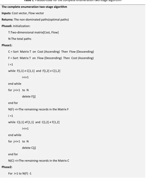
Table 1: Pseudo-code for the complete enumeration two-stage algorithm
The complete enumeration two-stage algorithm
Inputs: Cost vector, Flow vector
Returns: The non-dominated paths(optimal paths)
Phase0. Initialization:
T:Two-dimensional matrix[Cost, Flow]
N:The total paths
Phase1:
C = Sort Matrix T on Cost (Ascending) Then Flow (Descending)
F = Sort Matrix T on Flow (Descending) Then Cost (Ascending)
i =1
while F*i,1+ ≠ C*1,1+ and F*i,2+ ≠ C*1,2+
i=i+1
end while
for j=i+1 to N
delete F[j]
end for
N(F) =i=The remaining records in the Matrix F
i =1
while C*i,1+ ≠F*1,1+ and C*i,2+ ≠ F*1,2+
i=i+1
end while
for j=i+1 to N
delete C[j]
end for
N(C) =i=The remaining records in the Matrix C
Phase2:
For j=i+1 to N(F)
If C[j,2] <= C[ i,2] then
Delete C[j]
End If
End For
End For
The remaining records are non-dominated solutions(optimal paths)
For i=1 to N(C) -1
For j=i+1 to N(C)
If F[j,1] >= F[ i,1] then
Delete F[j]
End If
End For
End For
The remaining records are non-dominated solutions(optimal paths)
Start the first phase of the algorithm
Initialization & Identification of Parameters
Generate a random network and define the number of nodes
Find all paths of the network and store them in a file
Find a path with the maximum flow in the network and its cost, as well as finding the path with the minimum cost and its flow.
Eliminate all paths out of the boundaries marked by the two paths
found at previous step.
Find paths which their boundaries have been specified according to fig.2.
Save Opt-path file and end of the first
Fig.1: Flowchart of the complete enumeration two-stage algorithm. Start the second
phase the algorithm
Flow i>Flow j
Flow i =Flow j Cost i ≤Cost j
Eliminate path i&
replace pathi with
path i& j
Eliminate path j&
replace path j with
path i Cost i ≤ cost j
End
Initialization & Identification of Parameters
Call a path from opt-path file of the first phase of the algorithm
Continue calling the paths until the opt-pat-file comes to its end
End of
opt-path file Print path i
Print both of
path i&j Print path i
Cost i ≥Cost
j
Print path j Print both
of path i&j
No
Yes
No
Yes
Yes
No No
Yes Yes
No
Yes
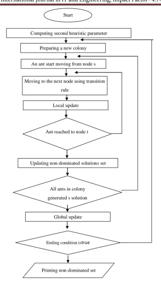
3.2. The ant colony optimization algorithm
The suggested ant colony algorithm is composed of some main functions such as pheromone matrix, heuristic parameter, evaporation, local update and global update. These functions are described in this section. The algorithm is designed based on classic ACS proposed by Dorigo and Gambardella with maximum selection in transition rule as well as local and global update. Fig. 2 presents a flowchart for the steps involved in the algorithm. For more details refer to (Ghoseiri andNadjari,2010: 1237-1246).
4. The application of the two algorithms to the problem
Fig. 2: Flowchart of the ant colony algorithm. Start
Computing second heuristic parameter
Preparing a new colony
An ant start moving from node s
Moving to the next node using transition
rule
Local update
Global update Ant reached to node t
All ants in colony
generated s solution
Updating non-dominated solutions set
Ending condition istrue
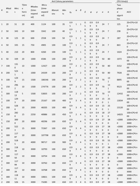
Table 2.Summary of results for the experimental analysis on instance problems.
# #Nod es #Arc s T(tim e horiz on) #Nodes (time-expand ed) #Arcs (time-expand ed)
Ant Colony parameters CPU time(s)
#Iterati ons
#An ts 𝑞0
α
β
δ φ ρ a b
Two phase d algorit hm ACO
1 20 51 20 400 1124 100 35 0.9 5 1 1
0. 5
0.9 9
0.9
9 24 7 125
20<CPU<10 0 2 50 343 10 500 3342 100 40 0.9
5 1 1 0. 5
0.9 9
0.9
9 24 7 238
20<CPU<10 0 3 30 125 20 600 2558 100 50 0.9
5 1 1 0. 5
0.9 9
0.9
9 24 7 287
20<CPU<10 0 4 50 335 15 750 4905 100 100 0.9
5 1 1 0. 5
0.9 9
0.9
9 24 7 863
20<CPU<10 0 5 40 210 20 800 4260 100 100 0.9
5 1 1 0. 5
0.9 9
0.9
9 24 7 1024
20<CPU<10 0 6 50 339 20 1000 6586 100 200 0.9
9 2 2 0. 1
0.9 9
0.9
9 50 80 1073
100<CPU<8 00 7 100 131
0 10 1000 12427 100 200 0.9 9 2 2
0. 1
0.9 9
0.9
9 50 80 3152
100<CPU<8 00 8 200 523
1 5 1000 24339 100 200 0.9 9 2 2
0. 1
0.9 9
0.9
9 50 80 7928
100<CPU<8 00 9 100 129
9 15 1500 186546 100 200 0.9 9 2 2
0. 1
0.9 9
0.9 9 70
13
1 8895
100<CPU<8 00 1
0 150 296
2 10 1500 274776 100 200 0.9 9 2 2
0. 1
0.9 9
0.9 9 70
13
1 9523
100<CPU<8 00 1
1 300 118
13 5 1500 53835 100 200 0.9 9 2 2
0. 1
0.9 9
0.9 9 70
13
1 12432
100<CPU<8 00 1
2 100 129
3 20 2000 25167 100 400 0.9 9 3 4
0. 1 0.9 9 0.9 9 15 0 25
1 13034
100<CPU<8 00 1
3 200 528
6 10 2000 48205 100 400 0.9 9 3 4
0. 1 0.9 9 0.9 9 15 0 25
1 13120
100<CPU<8 00 1
4 150 282
0 15 2250 40886 100 450 0.9 9 2 4
0. 1 0.9 9 0.9 9 18 0 27
0 14025
100<CPU<8 00 1
5 150 300
0 20 3000 40296 100 650 0.9 9 3 4
0. 1 0.9 9 0.9 9 27 0 38 0 >2000 0 1000<CPU< 3000 1
6 200 522
3 15 3000 72367 100 650 0.9 9 3 4
0. 1 0.9 9 0.9 9 27 0 38 0 >2000 0 1000<CPU< 3000 1
7 300 117
87 10 3000 107798 100 650 0.9 9 3 4
0. 1 0.9 9 0.9 9 27 0 38 0 >2000 0 1000<CPU< 3000 1
8 200 518
5 20 4000 98717 100 900 0.9 9 2 4
0. 1 0.9 9 0.9 9 35 0 55 1 >2000 0 1000<CPU< 3000 1
9 300 118
34 10 3000 10793 100 650 0.9 9 3 4
0. 1 0.9 9 0.9 9 27 0 38 0 >2000 0 1000<CPU< 3000 2
0 300 117
50 10 3000 10754 100 650 0.9 9 3 4
0. 1 0.9 9 0.9 9 27 0 38 0 >2000 0 1000<CPU< 3000 2
1 300 117
99 10 3000 10762 100 650 0.9 9 3 4
0. 1 0.9 9 0.9 9 27 0 38 0 >2000 0 1000<CPU< 3000 2
2 300 117
39 10 3000 10768 100 650 0.9 9 3 4
0. 1 0.9 9 0.9 9 27 0 38 0 >2000 0 1000<CPU< 3000 2
3 300 118
11 10 3000 10821 100 650 0.9 9 3 4
4 4 9 1 9 9 0 0 0 3000 2
5 200 522
3 15 3000 72198 100 650 0.9 9 3 4
0. 1 0.9 9 0.9 9 27 0 38 0 >2000 0 1000<CPU< 3000 2
6 200 518
8 15 3000 70753 100 650 0.9 9 3 4
0. 1 0.9 9 0.9 9 27 0 38 0 >2000 0 1000<CPU< 3000 2
7 200 520
1 15 3000 72252 100 650 0.9 9 3 4
0. 1 0.9 9 0.9 9 27 0 38 0 >2000 0 1000<CPU< 3000 2
8 200 523
7 15 3000 73346 100 650 0.9 9 3 4
0. 1 0.9 9 0.9 9 27 0 38 0 >2000 0 1000<CPU< 3000 2
9 200 514
8 20 4000 97654 100 900 0.9 9 2 4
0. 1 0.9 9 0.9 9 35 0 55 1 >2000 0 1000<CPU< 3000 3
0 200 516
6 20 4000 98852 100 900 0.9 9 2 4
0. 1 0.9 9 0.9 9 35 0 55 1 >2000 0 1000<CPU< 3000 3
1 200 516
9 20 4000 98293 100 900 0.9 9 2 4
0. 1 0.9 9 0.9 9 35 0 55 1 >2000 0 1000<CPU< 3000 3
2 200 527
1 20 4000 100706 100 900 0.9 9 2 4
0. 1 0.9 9 0.9 9 35 0 55 1 >2000 0 1000<CPU< 3000 3
3 200 517
1 20 4000 98078 100 900 0.9 9 2 4
0. 1 0.9 9 0.9 9 35 0 55 1 >2000 0 1000<CPU< 3000
A set of 33 acyclic network problems ranging from 400 to 4000 nodes are solved and results are compared with solutions produced by the two-phased exact algorithm . Table 2 shows specifications and comparison results and includes parameter values used to solve the instance problems where #Nodes and #Arcs denotes the number of nodes and arcs in origin network, respectively and #Nodes (time-expanded) and #Arcs (time-expanded) denotes the number of nodes and arcs in time-expanded network, respectively. T denotes the time horizon and #ants indicates number of ants in colony and #iterations indicates number of algorithm iterations (colonies). The parameters q0,α,β,δ,φ,ρ, a and bdenote the selection parameter in ant colony transition rule, preference weight of pheromone trail, preference weight of the first heuristic parameter, preference weight of the second heuristic parameter, local update evaporation rate, global update evaporation rate, respectively (Ghoseiri andNadjari, 2010: 1237-1246).
Parameter 𝑎 identifies the number of ants that use only information of the second objective and finally CPU denotes the average CPU time in seconds. The number of iterations (colonies) in all runs considered equal to 100. The number of iterations considered fix in all runs and varied number of ants in colonies regarding the size of problem. Increasing the number of nodes and arcs in network make the algorithm uses more ants to search in larger space. The selection parametersq0, weighting parameters α,β and δ and also updating parameters φ and ρ are experimental values and would be set experimentally. Ghoseiri et al. considered these parameters in the first run of the algorithm respectively set equal to 0.99, 2, 4, 1, 0.9999 and 0.99 and we use these numbers for the first run of the algorithm and in the second and third run they are changed in a way that better solutions are reached (Ghoseiri andNadjari, 2010: 1237-1246).
5. Conclusions
The present study has focused on the bi-criteria dynamic network. First, the bi-criteria dynamic network was converted into a time-phased network as. Then, two objectives were determined for the converted network. The first is maximizing the flow of traversing through the paths and the second deals with obtaining all shortest paths. The above objectives conflict with each other and generally lead to generating the dominated paths. In this research, two algorithms were used to obtain the non-dominated paths by which 33 generated random instances were solved. First using a two-stage complete enumeration algorithm the non-dominated paths generated. Then these solutions were compared with ACO algorithm.Computational results show that for problems with greater sizes (more than 800 nodes in time-expanded network), CPU time of the ACO algorithm is much smaller than the complete enumeration algorithm. In other word, the results on the set of instance problems show that the used ACO algorithm time saving in computation of large-scale bi-criteria shortest path problems.
References
R.K. Ahuja, M. Magnanti, J. Orlin," Network Flows. Theory, Algorithms and Applications, Prentice-Hall, Englewood Cliffs, New Jersey. (1993)
SaharAbbasi, S.Ebrahimnejad, The cross-entropy method for solving bi-criteria network flow problems in discrete-time dynamic networks, Optimization Methods & Software.2014,1-19.
L. R. Ford and D. R. Fulkerson.Constructing maximal dynamic flows from static flows.OperationsResearch , 6:419–433, 1958.
L. R. Ford and D. R. Fulkerson.Flows in Networks.Princeton University Press, Princeton, NJ, 1962. R.E. Bellman. On a routing problem. Quarterly of Applied Mathematics 16,87–90., 1958.
RBatta, S.S.Chiu. Optimal obnoxious paths on a network: Transportation of hazardous materials. Operations Research 36, 84–92.1988.
Current, J.R., Min, H., 1986.Multiobjective design of transportation networks: Taxonomy and annotation. European Journal of Operational Research 26, 187– 201.
Current, J.R., Marsh, M., 1993.Multiobjective transportation network design and routing problems: Taxonomy and annotation. European Journal of Operational Research 103, 426–438.
L.Cooke, ,E.Halsey,: The shortest route through a network with time-dependent intermodal transit times. J. Math. Anal.Appl. 14, 492–498 (1966).
EbrahimNasrabadi , S. Mehdi Hashemi, "Minimum cost time-varying network flow problems", Optimization Methods and Software, Volume 25, Issue 3: pages 429-447, 2010.
F. Guerriero & L. Di Puglia Pugliese,”Multi-dimensional labeling approaches to solve the linear fractional elementary shortest path problem with time windows”, Optimization Methods and Software ,Volume 26, Issue 2: pages 295-340, 2011.
Luigi Di Puglia Pugliese, Francesca Guerriero," Dynamic programming approaches to solve the shortest path problem with forbidden paths", Optimization Methods and Software, Version of record first published: 21 Nov 2011.
C. Chitra, P. Subbaraj.,Anondominated sorting genetic algorithm solution for shortest path routing problem in computer networks, Expert Systems with Applications 39 , 1518–1525 (2012).
H.He, G.Song,” Optimal paths in dynamic networks with dependent random link travel times”,Transportation Research Part B, 46 , 579–598.2012.
M. Dorigo, V. Maniezzo, A. Colorni, Ant System: An Autocatalytic Optimizing Process, Technical Report, Dipartimento di Elettronica e Informazione, Politecnico di Milano, 1991.
M. Dorigo, L.M. Gambardella, A cooperative learning approach to the traveling salesman problem, IEEE Transaction on Evolutionary Computation 1 (1997).53–66
KeivanGhoseiri, BehnamNadjari: An ant colony optimization algorithm for the bi-objective shortest path problem. Appl. Soft Comput. 10(4): 1237-1246 (2010).