Comparative Analysis of Biogeography-Based
Optimization and Fuzzy Logic in Load
Frequency Control
Hatef Farshi
1, Khalil Valipour
2M.Sc., Department of Electrical Engineering, Mohaghegh Ardabili University, Ardabil, Iran1
Assistant Professor, Department of Electrical Engineering Department, Mohaghegh Ardabili University, Ardabil, Iran2
ABSTRACT: Load Frequency Control (LFC) is one of the vital parts in power system design, automation, operation and stability.In this paper, we compare two different controllers,the Biogeography-Based Optimization (BBO) based PID controller and Fuzzy Logic Controller (FLC), in LFC problem of two area interconnected hydrothermal power system. The hydro and thermal areas are comprised with an electric governor and reheat turbine, respectively.Also, 1% Step Load Perturbation (SLP) has been considered in any individual area. The mentioned power system with the proposed approach is simulated in MATLAB/SIMULINK and the responses of frequency and tie-line power deviation for these two controllers in each area were shown and compared. The simulation results show that FLC achieves better responses in comparison with BBO based PID controller.
KEYWORDS:Load Frequency Control (LFC), PID controller, Bio-geography Based Optimization (BBO), Fuzzy Logic Controller (FLC), Step Load Perturbation (SLP), Integral Square Error (ISE)
I. INTRODUCTION
Modern power systems are interconnected units which the electrical power is transferred between them. Load Frequency Control (LFC) plays a great role in power system operation and stability because of its duty to preserve frequency and transferred power in their scheduled value, in normal condition and in the case of a very slight perturbation of the load. Generally LFC is a control system with three main purposes as follows:
Preserving system frequency in nominal value or close to it. Preserving the transferred power in a scheduled value.
Preserving each unit generation in an economically suitable value [1]-[4].
The first and second aims of LFC is frequency regulation to nominal value and preserving power transfer between the control areas by changing output of selected generators. The third aim is to distribute the needed change between generations of the units, so the operation cost will decrease.
When the load increases (decreases), the turbine’s velocity will decrease (increase) until the governor could coordinate the incoming steam with the new load. The less changes of the velocity will result in less error.
One way to restore nominal values of the velocity or the frequency is to add a controller (PI, PID, fuzzy logic and artificial neural network controller) to the system. These controllers will detect the average value of error and overcome the deviation.
Since the power system load change is continuous, generation control is set to automatic state to restore nominal values of frequency.
It is obvious that frequency is related to active power (P) and any change of power is influenced by system frequency. An optimal power system should tolerate sudden changes of load and preserve voltage and frequency in an acceptable range [5]-[8].
II. SYSTEM MODELLING
A. Two-area LFC Model
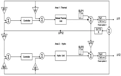
Generally, power system consists of several subsystems interconnected through tie lines. The investigated LFC system, in this paper, consists of two hydro-thermal areas. Area 1 is reheat thermal system and area 2 is hydro system. The hydro area is comprised with an electric governor and thermal area is comprised with reheat turbine. 1% step load perturbation is considered in both thermal and hydro area.
The generalized model of two-area interconnected power system is shown in figures 1. Also, nomenclature for various symbols is given after appendix.
Fig. 1. Investigated two-area power system.
B. Thermal Unit
The thermal unit of investigated two-area power system consists of governor and steam turbine with reheater. Dynamic model of this thermal area is shown in figure 2.
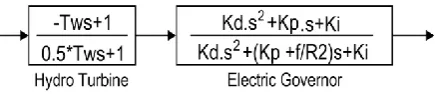
C. Hydro Unit
The hydro area of investigated power system includes electric governor and hydro turbine. Dynamic model of this hydro area is shown in figure 3.
Fig. 3. Dynamic model of hydro area.
III. BBO BASED PID CONTROLLER
BBO is an evolutionary algorithm that uses the mathematical models and concepts of the biogeography. These models describe migration of species between habitats in an ecosystem and how species arise or disappear. BBO, introduced by Dan Simon in 2008 [9], is a population-based global optimization algorithm inspired by the science of biogeography. In BBO, each possible solution is considered as a habitat and their features that characterize habitability are called Suitability Index Variables (SIV). The goodness of each solution is called its Habitat Suitability Index (HSI), where a high HSI of an island means good performance on the optimization problem, and vice versa.
The method to generate the next generation in BBO is by immigrating solution features to other islands, and receiving solution features by emigration from them.
The immigration rate and emigration rate of the jth island can be formulated as follows [10]:
𝜆𝑆𝑗 = 𝐼𝑚(1 − 𝑆𝑗
𝑆𝑚𝑎𝑥) (1)
𝜇𝑆𝑗 =𝐸𝑚 . 𝑆𝑗
𝑆𝑚𝑎𝑥 (2)
Where 𝜆𝑠𝑗 and 𝜇𝑠𝑗 are the immigration and emigration rates; 𝐼𝑚 is the maximum possible immigration rate; 𝐸𝑚 is the maximum possible emigration rate; 𝑆𝑗 is the number of species; and 𝑆𝑚𝑎𝑥 is the maximum number of species. Mutation operator modifies a habitat's SIV randomly based on mutation rate. The mutation rate 𝑚𝑠𝑗 is expressed as
(3).
𝑚𝑆𝑗 = 𝑚𝑚𝑎𝑥(1−𝑃𝑆𝑗
𝑃𝑚𝑎𝑥 ) (3)
Where 𝑚𝑚𝑎𝑥 is the maximum mutation rate; 𝑃𝑚𝑎𝑥 is the maximum species count probability; 𝑃𝑆𝑗 is the species count probability which is given by (4).
𝑃𝑆𝑗 =
− 𝜆𝑆𝑗 + 𝜇𝑆𝑗 𝑃𝑆𝑗+ 𝜇 𝑆+1 𝑗𝑃 𝑆+1 𝑗𝑆 = 0
− 𝜆𝑆𝑗 + 𝜇𝑆𝑗 𝑃𝑆𝑗 + 𝜆 𝑆−1 𝑗𝑃 𝑆−1 𝑗+ 𝜇 𝑆+1 𝑗𝑃 𝑆+1 𝑗1 ≪ 𝑆 ≪ 𝑆𝑚𝑎𝑥 − 1
− 𝜆𝑆𝑗+ 𝜇𝑆𝑗 𝑃𝑆𝑗 + 𝜆 𝑆−1 𝑗𝑃 𝑆−1 𝑗 𝑆 = 𝑆𝑚𝑎𝑥
(4)
Where 𝜇 𝑆+1 𝑗 and 𝜆 𝑆−1 𝑗 are the emigration and immigration rates for the j
th habitat contain (s+1) and (s-1) number of
species, respectively.
Define the problem, variables and select BBO parameters (number of habitats, immigration rate (λ), mutation rate (m), and emigration rate (µ))
Initialize the habitats
Modify habitats (migration) based on λ, µ Mutation
If termination criteria is reached, End. Otherwise go to step 3 for next iteration [10],[ 11].
In spite of many complicated control theories and techniques, more than 90% of control strategies still use PID controllers. This is mainly because of structural simplicity, high reliability, good stability and the convenient ratio between performances and cost of PID controller [12],[13].
A typical structure of a PID controller includes three separate elements: the proportional, integral and derivative values. So, BBO technique is used to optimize the PID parameters by Integral Square Error (ISE) criteria (Equation 5) in this paper.
J = ∫ (∆𝑓12+ ∆𝑓12+ ∆𝑃𝑡𝑖𝑒2) (5)
∆Ptie and ∆f are tie-line power and frequency deviations, respectively.
The effect of PID controller parameters on a closed loop system is summarized in the table 1.
Table 1.Effect of PID parameters.
Parameter Rise time Overshoot Settling time Steady state error
kp Decrease Increase Small change Decrease
ki Decrease Increase Increase Eliminate
kd Small change Decrease Decrease No change
IV. FUZZY LOGIC CONTROLLER
Since power system dynamic characteristics are complex and variable, conventional control methods cannot provide good results. Intelligent controller can be replaced with conventional controller to get fast and good dynamic response in load frequency problems. FLC can be more useful in solving large scale of controlling problems in comparison with conventional controllers. FLC is designed to minimize fluctuation on system outputs (∆f1, ∆f2 and ∆Ptie). There are many studies on LFC of power system with fuzzy logic controller like [14],[15].
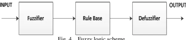
A FLC consist of three sections namely fuzzifier, rule base and defuzzifier as shown in figure 4.
Fig. 4. Fuzzy logic scheme.
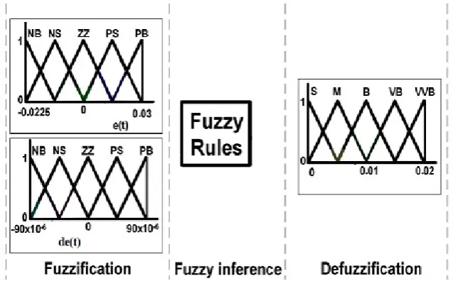
Five membership functions are used in both inputs and output of this fuzzy system which are as follows:
Positive Big (PB), Positive Small (PS), Zero (Z), Negative Small (NS), Negative Big (NB), Small (S), Medium (M), Big (B), very Big (VB), Very Very Big (VVB).
Table 2. Fuzzy rules.
d (ACE)
NB NS Z PS PB
ACE
NB S S M M B
NS S M M B VB
Z M M B VB VB
PS M B VB VB VVB
PB B VB VB VVB VVB
Figure 5 shows this fuzzy system briefly.
Fig. 5. Fuzzy inference system for LFC.
V. RESULTS AND ANALYSIS
Table 3. PID controllers' parameters.
BBO
kp1 0.492908
ki1 0.730713
kd1 0.358271
kp2 0.428614
ki2 0.176308
kd2 0.137494
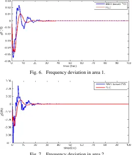
Dynamic responses of frequency deviation by these two methods are shown in figures 6 and 7.
Fig. 6. Frequency deviation in area 1.
Fig. 7. Frequency deviation in area 2.
Fig. 8. Tie-line power deviation.
Cost function of BBO is shown in figure 9.
Fig. 9. BBO cost function.
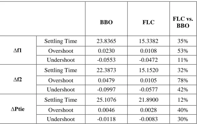
The detailed information for frequency and tie-line power deviation of area 1 and 2 is shown in table 4 for two mentioned methods.
Table 4. Detailed information for frequency and tie-line power deviation.
BBO FLC FLC vs.
BBO
∆f1
Settling Time 23.8365 15.3382 35%
Overshoot 0.0230 0.0108 53%
Undershoot -0.0553 -0.0472 11%
∆f2
Settling Time 22.3873 15.1520 32%
Overshoot 0.0479 0.0105 78%
Undershoot -0.0997 -0.0577 42%
∆Ptie
Settling Time 25.1076 21.8900 12%
Overshoot 0.0046 0.0028 40%
By observing the above tables, we can conclude the FLC is more robust than BBO based PID controller.
In ∆f1, ∆f2 and ∆Ptie, the settling time of FLC has about 35%, 32% and 12% improvement in comparison with BBO, respectively. Also, Overshoot response of FLC has about 53%, 78% and 40% improvement. There are almost 11, 42 and 30 percent improvement for undershoot of it, too.
VI. CONCLUSIONS
In this paper, the PID controller has employed for LFC of two-area interconnected hydro-thermal power system and its parameters have determined by a metaheuristic algorithm (BBO). Furthermore, FLC has used in this power system. Then, LFC model by these two mentioned controllers has simulated in MATLAB/SIMULINK and their results have compared with each other. It has shown in section 5 that FLC has superiority in comparison with BBO based PID controller. APPENDIX Value Parameter 60 Hz f 1, 2 i 2000MW Pri 5sec Hi
8.33*10-3 Pu MW/ Hz D1
12.5*10-3 Pu MW/ Hz D2
0.086 Pu MW/radians T12
2.4 Hz/Pu MW Ri 0.08 sec Tg 0.5 Kr 10 sec Tr 0.3 sec Tt 0.424 Bi 20 sec Tp1 13 sec Tp2
120 Hz/Pu MW Kp1
80 Hz/Pu MW Kp2 4 Kd 1 Kp 5 Ki 1 sec Tw -1 a12 0.01 SLP NOMENCLATURES
f :Nominal system frequency
i:Subscript referred to area i
Hi:Inertia constant
D1:∆PD1/ ∆f1 D2:∆PD2/ ∆f2
T12:Synchronizing coefficient
Ri:Governor speed regulation parameter Tg:Steam governor time constant Kr:Steam turbine reheat constant Tr:Steam turbine reheat time constant Tt:Steam turbine time constant Bi:Frequency bias constant Tp1:2Hi/f*D1
Tp2:2Hi/f*D2 Kp1:1/D1 Kp2:1/D2
Kd:Electric governor derivative gain Kp:Electric governor proportional gain Ki:Electric governor integral gain Tw:Water starting time
∆fi:Frequency deviation of area i
∆Ptie(∆P12):Tie-line power deviation
ACEi:Area control error of area i (Bi∆fi±∆Ptie) a12:−Pr1/Pr2
J:Cost index
SLP:Step load perturbation
REFERENCES
[1] H. Shabani, B. Vahidi, M.A. Ebrahimpour, “A robust PID controller based on imperialist competitive algorithm for load-frequency control of power systems”, ISA Transactions, Vol. 52, pp. 88–95, 2013.
[2] H. Saadat, “Power system analysis”, USA: McGraw-Hill; 1999.
[3] Kundur, “Power system stability and control”, New York: Mc-Grall Hill; pp. 601–623, 1994.
[4] H. Bevrani, T. Hiyama, “Intelligent automatic generation control”, Taylor & Francis Group, USA, pp.11–36, 2011.
[5] D.G. Padhan, S. Majhi, “ A new control scheme for PID load frequency controller of single -area and multi-area power systems”, ISA Transactions, Vol. 52, pp. 242–251, 2013.
[6] H. Shayeghi, H.A. Shayanfar, A. Jalili, “Load frequency control strategies: A state-of-the-art survey for the researcher”, Energy Conversion and Management, Vol. 50, pp. 344–353, 2009.
[7] Ibraheem, P. Kumar P, Kothari,“ Recent philosophies of automatic generation control strategies in power systems”, IEEE Transaction on Power System, Vol. 20, pp. 346–357, 2005.
[8] S.K. Pandey, S.R. Mohanty, N. Kishor, “ A literature survey on load–frequency control for conventional and distribution generation power systems”, Renewable and Sustainable Energy Reviews, Vol. 25, pp. 318–334, 2013.
[9] D. Simon, “Biogeography-Based Optimization”, IEEE Transaction on Evolutionary Computation, Vol. 12, No. 6, 2008.
[10] P.K. Ammu, K.C. Sivakumar, R. Rejimoan, “Biogeography-Based Optimization - A Survey”, International Journal of Electronics and Computer Science Engineering, Vol. 2, No. 1, pp. 154–160, 2013.
[11] H. Kumar, S. Ushakumari, “Biogeography based Tuning of PID Controllers for Load Frequency Control in Microgrid”, International Conference on Circuit, Power and Computing Technologies, pp. 797–802, 2014.
[12] L. Santos Coelho, V.C. Mariani, “Firefly algorithm approach based on chaotic Tinkerbell map applied to multivariable PID controller tuning”, Computers and Mathematics with Applications, Vol. 64, pp. 2371–2382, 2012.
[13] R. Kumar Sahu, S. Panda, S. Padhan, “A hybrid firefly algorithm and pattern search technique for automatic generation control of multi area power systems”, Electrical Power and Energy Systems, Vol. 64, pp. 9–23, 2015.
[14] H. Guolian, Q. Lina, Z. Xinyan, Z. Jianhua, “ Application of PSO-Based Fuzzy PI Controller in Multi-area AGC System after Deregulation”, IEEE Conference on Industrial Electronics and Applications, Vol. 7, pp. 1417–1422, 2012.
BIOGRAPHY
Hatef Farshiwas born in Meshkin Shahr, Iran, 1990. He received the B.Sc. degree of electrical engineering from Islamic Azad University-Ardabil Branch in 2013. He is currently the M.Sc. student at department of electrical engineering in Mohaghegh Ardabili University.His research interests include application of artificial intelligence in power systems, power system dynamics, renewable energy and distributed generation.