Volume 2010, Article ID 579295,20pages doi:10.1155/2010/579295
Review Article
Time-Frequency Analysis and Its Application in
Digital Watermarking
Srdjan Stankovi´c
Faculty of Electrical Engineering, University of Montenegro, 20000 Podgorica, Montenegro
Correspondence should be addressed to Srdjan Stankovi´c,[email protected]
Received 14 February 2010; Accepted 7 June 2010
Academic Editor: Sridhar Krishnan
Copyright © 2010 Srdjan Stankovi´c. This is an open access article distributed under the Creative Commons Attribution License, which permits unrestricted use, distribution, and reproduction in any medium, provided the original work is properly cited.
A review of time-frequency analysis and some aspects of its applications in digital watermarking are presented. The main advantages and drawbacks of various time-frequency distributions are first discussed. The aim of this theoretical overview is to facilitate an appropriate distribution selection in a specific application. Different aspects of the time-frequency analysis when applied to digital watermarking are then presented. In particular, the method that maps time-frequency characteristics of a host signal to the pseudo noise watermark sequence is thoroughly discussed. This approach is presented in the multidimensional form and then applied to digital audio, digital image, and digital video watermarking. Finally, the theoretical considerations are illustrated by various numerical and real-life examples.
1. Introduction
Theoretical aspects of time-frequency analysis have been intensively studied over the last two decades [1–27]. In par-allel, their various applications have been exploited as well. Namely, for an efficient analysis of nonstationary signals, such are radar, sonar, biomedical, seismic, and multimedia signals, time-frequency representations are required. Time-frequency distributions are most commonly used for this purpose. Many of the researchers have made significant efforts in defining a distribution that is optimal for a wide class of frequency-modulated signals [8–11]. As a result, a number of time-frequency distributions have been proposed. However, the efficiency of each of them is more or less limited to a specific class of signals and, consequently, to a specific application. One of the goals of this paper is to highlight the most important features of some popular time-frequency distributions and to give an idea of how to choose the most appropriate distribution depending on the signal form. The linear, quadratic, higher-order, and multiwindow time-frequency distributions are considered. The short-time Fourier transform, as the most commonly used linear transform, is firstly discussed. Next, the Wigner distribution, as the best known quadratic distribution, is presented. Also, the Cohen class and some specific distributions belonging
to this class are considered [1, 5–7]. It is shown that the quadratic distributions are optimal for a linear frequency-modulated signal. However, if the instantaneous frequency variation within the analysis window is faster, multiwindow, or higher order distributions should be used, [14–16,19–27]. The Hermite functions-based multiwindow approach is also discussed. Finally, highly concentrated distributions with complex-lag argument are presented. To facilitate in better understanding of the presented theoretical considerations, numerous illustrative examples have been provided.
−2 0 2
0 100 200 300
Time Signal
−2 0 2
0 100 200 300
Time Signal
(a) (a)
0 50 100
0 50 100 150
Frequency
Fourier transform modulus
0 50 100
0 50 100 150
Frequency
Fourier transform modulus
(b) (b)
60 40 20
Fre
q
u
en
cy
50 100 150 200 250 300
Time
Time-frequency representation
60 40 20
50 100 150 200 250 300
Fre
q
u
en
cy
Time
Time-frequency representation
(c) (c)
Figure1: Nonstationary signals. (a) Time domain representations. (b) Fourier domain representations. (c) Spectral components’ variations along the time axes.
the host signal. The detection is performed in the time-frequency domain. This particular approach is presented in the multidimensional form, and it is applied to digital audio, digital image, and digital video. It provides a high degree of robustness and imperceptibility. Hence, even when the watermark is very weak, a reliably detection can still be achieved. Also, the watermark gets completely hidden by the time-frequency characteristics of the host signal.
2. Time-Frequency Analysis
The Fourier transform provides spectral content of a signal. It has been a valuable tool in various applications. However, for nonstationary signals the Fourier transform cannot give satisfactory results since the information about frequency components variations in time is required.
Furthermore, it can happen that two different signals have the same spectral contents, as illustrated in Figures1(a)
and1(b). Based on Figure 1(c), however, we can conclude
that the time-frequency representations of the two signals are quite different. This example is a simple illustration of the importance of time-frequency analysis for signals whose spectral contents vary with time. Various time-frequency distributions are used for this purpose. The ideal time-frequency representation can be described as [19–21]
ITF(t,ω)=2πA2δ(ω−Φ(t)), (1)
where a signal of the formx(t)=AejΦ(t)is considered. This
representation provides the signal local energy distribution, as well.
A question that naturally arises at this point is whether there exist a single representation that would be ideal for any signal at hand. The answer is no, hence a number of time-frequency distributions have been introduced.
s(t) w(τ) Sliding t FT { s ( t1 + τ ) w ( τ ) } FT { s ( t2 + τ ) w ( τ ) } FT { s ( ti + τ ) w ( τ ) } FT { s ( tN + τ ) w ( τ ) } Fre q u en cy
t1t2 ti tN
Time Figure2: Illustration of the STFT calculation.
obtained by using the short-time Fourier transform (STFT) defined as [2]
STFT(t,ω)=
∞
−∞x(t+τ)w(τ)e
−jωτdτ. (2)
Thus, it is a windowed version of the Fourier transform. The sliding window function is denoted byw(τ), whereτis the lag coordinate. An illustration of the STFT calculation is shown inFigure 2.
Note that the spectral content is calculated for each windowed part of the signal. The central point of the sliding window is the time instant for which the spectrum is calculated. The influence of the window size is critical, as it will be discussed later.
The energetic version of the STFT is known as the spectrogram. It can be written as
SPEC(t,ω)= |STFT(t,ω)|2
=2πA2W(ω−Φ(t))∗ ωFT
ej(Q(t,τ), (3)
where W(ω) is the Fourier transform of the time domain window w(t), Φ(t) is the first derivative of the phase function, the frequency convolution is denoted by ∗ω, while Q(t,τ)=Φ(2)(t)(τ2/2!) +Φ(3)(τ3/3!) +· · ·+Φ(n)(τn/n!) is the spread factor which depends on the second and higher order phase derivatives. Note that an ideal representation will be obtained if the signal is constant frequency modulated (Φ(i)(t)=0, for i≥2) and ifW(ω−Φ(t)) → δ(ω−Φ(t)), that is, for a large time domain window. However, if the signal is not constant frequency modulated, a large window size can produce a low time resolution and vice versa. In general, there is a trade-offbetween the time and frequency resolution, and it is best described with the uncertainty principle, as
MTMw≥ 1
2, (4)
where,
MT=
∞
−∞ τ2|w(τ)|2dτ ∞
−∞|w(τ)|2dτ
, Mw=
∞
−∞ ω2|W(ω)|2dω ∞
−∞|W(ω)|2dω (5)
are the measures of duration in time and frequency, respec-tively. The signal should satisfyw(t)√t →0 ast → ±∞.
An illustration of the window size influence on the spec-trogram resolution is given inFigure 3. A four-component signal is considered. In order to achieve a good time resolu-tion, two short sinusoidal components should be analyzed by using a narrow window. However, to obtain a good frequency resolution the third component (a sinusoid with a long duration) should be analyzed by using a wide window.
In Figure 3(a), a narrow window is used, and it results in
a good time resolution, while the frequency resolution is low. However, when a large window size is used, a low time resolution is obtained. Hence, the two short sinusoids have almost merged into one (seeFigure 3(b)). Due to the presence of a linear frequency-modulated component (chirp signal), the spread factors are present in both cases.
The spectrogram satisfies the marginal properties
t
SPEC(t,ω)dt= |X(ω)|2
,
1 2π
ω
SPEC(t,ω)dω= |x(t)|2
.
(6)
The total energy is obtained as
Ex= 1
2π
t
ω
SPEC(t,ω)dt dω. (7)
An important property of the STFT is its linearity. Namely, the STFT of a multicomponent signalx(t) = M
i=1xi(t) is
STFTx(t,ω)=M
i=1STFTxi(t,ω). Consequently, if the signal
components do not intersect in the time-frequency plane the spectrogram will be equal to the sum of spectrograms of each of the signal components. This is evident fromFigure 3.
2.2. Quadratic Time-Frequency Distributions. Quadratic time-frequency distributions have been introduced in order to improve the time-frequency resolution. Namely, they remove the spread factors for linear frequency-modulated signals. Among them, the Wigner distribution is the most commonly used. It has also been used as a base to define several interesting time-frequency distributions.
The windowed version of the Wigner distribution is called the pseudo-Wigner distribution. It is defined as [1,2]
WD(t,ω)
=
∞
−∞x
t+τ 2
x∗
t−τ
2 w τ 2 w∗ −τ 2
e−jωτdτ.
(8)
5 10 15 20
Fre
q
u
en
cy
25 30
500 1000 1500
Time Spectrogram
(a)
50 100 150 200 250
Fre
q
u
en
cy
500 1000 1500 2000
Time Spectrogram
(b)
Figure3: STFT of the four-component signal calculated by: (a) narrow window, (b) large window.
50 100 150 200 250
Fre
q
u
en
cy
500 1000 1500 2000
Time Wigner distribution
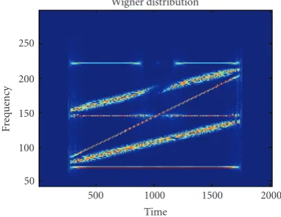
Figure4: Wigner distribution of a four-component signal.
The Wigner distribution satisfies the marginal condi-tions. Note that it is always real, while the numerical realization requires oversampling with factor 2. However, the Wigner distribution is not linear. Namely, for a multicompo-nent signalx(t)= M
i=1xi(t), the Wigner distribution is of
the form
WD(t,ω)=
M
i=1
WDxixi(t,ω) +
M
i=1
M
k=1
i /=k
WDxixk(t,ω). (9)
Thus, beside the autoterms, the interactions between dif-ferent signal components (WDxixk(t,ω)), called cross-terms,
appear. This is a major drawback of this distribution. The Wigner distribution of the four-component signal, from the previous example, is given inFigure 4.
In this case, the auto components are well concentrated. However, the cross-terms presence is significant. Namely, the time-frequency representation contains frequency compo-nents that do not exist within the signal itself. It could lead to a wrong analysis result.
The cross-terms could be reduced by using a filter function in the ambiguity domain. The ambiguity function is the two dimensional Fourier transform of the Wigner distribution, that is,
A(τ,θ)=FT2D{WD(t,ω)}. (10)
In the ambiguity domain, the auto-terms are located around the origin. Thus, a two-dimensional filter, called the kernel function, is used to filter out the cross-terms (that are generally located away from the origin) [1,5–7]:
Af(τ,θ)=A(τ,θ)c(τ,θ), (11)
where A(τ,θ) = −∞∞ x(t +τ/2)x∗(t −τ/2)e−jθtdt is the ambiguity function, and c(τ,θ) is the kernel function. The time-frequency distribution based on the filtered function is obtained as
CD(t,ω)=IFT{A(τ,θ)c(τ,θ)}
= 1
2π
∞
−∞c(τ,θ)x
u+τ 2
x∗
u−τ
2
×e−jθte−jωτejθudθ du dτ.
(12)
This is the definition of the Cohen class of distributions. By choosing the corresponding kernel functions, some specific distributions belonging to the Cohen class can be obtained. They satisfy the marginal properties if c(0,θ) = c(τ, 0) = 1 holds. For example, the Choi-Williams distribution [5] is obtained for the kernel functionc(τ,θ)=e−(τ2θ2/σ2)
whereσ is a scaling factor to control its attenuation rate. The kernels for some distributions are defined inTable 1, [7].
250 200 150 100 50
500 1000 1500
(a)
250 200 150 100 50
500 1000 1500
(b)
250 200 150 100 50
500 1000 1500
(c)
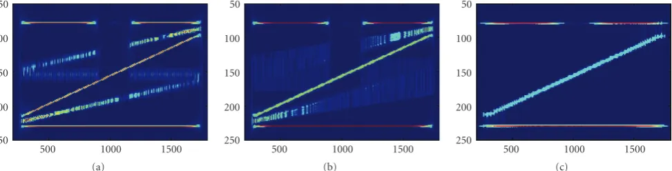
Figure5: Time-frequency representations by: (a) Choi-Williams distribution (σ=2π), (b) Born-Jordan distribution, and (c) Choi-Williams distribution (σ=0.5).
Table1: Some distributions from the Cohen class.
Distribution Kernel
Choi-Williams e−θ2τ2/σ2
Born-Jordan (sin(θτ/2))/θτ/2
Zao-Atlas-Marks |τ|(sin(θτ/2)/θτ/2)w(τ)
Sinc distribution rect(θτ/α)
Wigner distribution w2(τ/2)
producing almost the same auto-terms concentration is shown in Figure 5(b). Note that the side-lobes and cross-terms are more emphasized than in the Choi-Williams distribution withσ=2π[7]. However, if the Choi-Williams distribution with the attenuation parameter σ = 0.5 is used (Figure 5(c)), the cross-terms get suppressed, while the auto-term concentration becomes reduced (for the chirp component).
Note that there is a trade-off between the cross-terms reduction and auto-term concentration (it depends on parameters of the kernel function). Obviously, distributions belonging to the Cohen class lie in between the two extreme cases: the spectrogram that eliminates the cross-terms with a low auto-term concentration and the Wigner distribution that provides high resolution, but with emphatic cross-terms. It is possible to obtain an ideal time-frequency concentration only if signal dependent kernels are used [8,10].
Next, we can ask the following question. Is there a distribution that provides the auto-terms concentration as good as in the Wigner distribution, while eliminating the cross-terms like the spectrogram does? In order to define a distribution with these properties, let us start with the following relationship between the short-time Fourier transform and the Wigner distribution:
WD(t,ω)= 1
π
∞
−∞STFT(t,ω+θ)STFT
∗(t,ω−θ)dθ. (13)
Clearly, the convolution along the frequency axis improves the auto-terms concentration, but it introduces the cross-terms. Thus, the convolution should be performed only over the same auto-terms, avoiding different signal components being convolved. It can be performed by introducing a frequency domain window (seeFigure 6).
−θ −θ +θ +θ −θ −θ +θ +θ
1 1-2 2
ω
STFT(ω+θ)
STFT∗(ω−θ)
+θ +θ −θ −θ +θ +θ −θ −θ
1 2-1 2
ω1 ω2 ω
ω1 ω2
Figure6: Illustration of the STFTs convolution.
A distribution that allows for such convolution is called the S-method [17]. It is defined as
SM(t,ω)= 1
π
∞
−∞P(θ)STFT(t,ω+θ)STFT
∗(t,ω−θ)dθ. (14)
The frequency domain finite window is denoted by P(θ) (P(θ) = 0 for|θ| > L). Observe that for P(θ) =
πδ(θ) andP(θ) = 1 the spectrogram and the Wigner distribution are obtained, respectively.
The discrete version of the S-method is
SM(n,k)=
L
i=−L
STFT(n,k+i)STFT∗(n,k−i)
=SPEC(n,k)
+ 2 Re
⎧ ⎨ ⎩
L
i=1
STFT(n,k+i)STFT∗(n,k−i)
⎫ ⎬ ⎭.
(15)
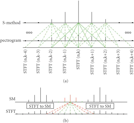
The discrete window width is 2L + 1. It determines the number of summation terms in (15). Note that they improve the spectrogram concentration toward that of the Wigner distribution. An illustration of the S-method calculation is shown inFigure 7.
S-method
Spectrogram
STFT
(n,k-4)
STFT
(n,k-3)
STFT
(n,k-2)
STFT
(n,k-1)
STFT
(n,k)
STFT
(n,k+1)
STFT
(n,k+2)
STFT
(n,k+3)
STFT
(n,k+4)
(a)
SM STFT
STFT to SM STFT to SM
(b)
Figure7: Illustration of the S-method calculation for a given time instantn.
7(b)). It is important to observe that the summation has to be performed only over the auto-terms. If the other terms are included, the concentration will not be improved. In addition, the noise could be also picked up. The window has to be narrower than the minimal distance between the auto-terms. If this is not the case, the interactions between the auto-terms will produce the cross-terms. Namely, as illustrated in Figure 7(b), the cross-terms appear if the window includes the summation terms marked by red color. The adaptive S-method with a variable window adjusted to the auto-terms is introduced in [18]. However, in many applications the fixed window size ofL=3 has been shown to provide very good results, since the convergence within the window is fast, and it is mostly achieved after a few summation terms.
The S-method of the four-component signal is given in
Figure 8.
Note that all signal components (with constant and linear frequency modulations) are well concentrated even forL =
3. By increasingL, forL >5 the cross-terms start to appear (the minimal distance between the auto-terms becomes less than 2L+ 1).
The spectrogram and the S-method (L = 3) of a real speech signal are shown inFigure 9.
The speech signal time-frequency resolution is improved by using the S-method.
Observe that the spread factor in the quadratic dis-tributions will be present if the instantaneous frequency contains third and higher order phase derivatives. Hence, further concentration improvement can be obtained by using the multiwindow approach or by using higher order time-frequency distributions, as discussed below.
2.3. Multiwindow Time-Frequency Distributions. The con-cept of multiwindow time-frequency distributions has been
developed by using optimally concentrated orthogonal win-dows [25–27]. The Hermite functions that are localized in both time and frequency domain can be used as orthogonal windows. The multiwindow spectrogram is defined as a weighted sum of the spectrograms:
SPECMW(t,ω)=
K−1
p=0
cp(t)SPECp(t,ω)
= 1
2π K−1
p=0
cp(t)
x(τ)Ψp(τ−t)e−jωτdτ2.
(16)
The total number of the spectrograms and Hermite functions isK, whilecp(t) are the weighting coefficients. Thepth order Hermite function is defined as
Ψp(t)=(−1)
p et2/2
2pp!√π
dpe−t2
dtp . (17)
This function can be obtained by using a recursive realization as follow
Ψp(t)=t
2 pΨp−1(t)
−
p−1
p Ψp−2(t), ∀p≥2,
(18)
while:
Ψ0(t)= √41πe −(t2/2)
, Ψ1(t)= √
2t
4
√
π e −(t2/2)
250 200 150 100 50
Fre
q
u
en
cy
500 1000 1500 2000
Time S-method (L=3)
(a)
250 200 150 100 50
Fre
q
u
en
cy
500 1000 1500 2000
Time S-method (L=5)
(b)
250 200 150 100 50
Fre
q
u
en
cy
500 1000 1500 2000
Time S-method (L=7)
(c)
250 200 150 100 50
Fre
q
u
en
cy
500 1000 1500 2000
Time S-method (L=16)
(d)
250 200 150 100 50
Fre
q
u
en
cy
500 1000 1500 2000
Time S-method (L=32)
(e)
250 200 150 100 50
Fre
q
u
en
cy
500 1000 1500 2000
Time S-method (L=64)
(f)
250 200 150 100 50
Fre
q
u
en
cy
500 1000 1500 2000
Time S-method (L=128)
(g)
250 200 150 100 50
Fre
q
u
en
cy
500 1000 1500 2000
Time S-method (L=256)
(h)
200 150 100 50
Fre
q
u
en
cy
100 200 300 400
Time Spectrogram
(a)
200 150 100 50
Fre
q
u
en
cy
100 200 300 400
Time S-method
(b)
Figure9: Time-frequency representations of a speech signal: (a) spectrogram, (b) S-method.
The weighting coefficients are calculated by
K−1
p=0
cp(t)
A2(t+τ)Ψ2
p(τ)τidτ
A2(t+τ)Ψ2p(τ)dτ = ⎧ ⎨ ⎩
1, fori=0
0, fori >0, (20)
where A(t) is the signal amplitude. The weighting coeffi -cients for a signal with a constant amplitude are given in
Table 2.
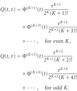
It is important to emphasize that the spread factor is reduced proportionally to the highest order of Hermite functions used in the multiwindow spectrogram:
Q(t,τ)=Φ(K+1)(t) τK+1
(K+ 1)!+Φ
(K+2)(t) τK+2
(K+ 2)!+· · · (21)
Thus, the first term in the spread factor comes from the (K+ 1)th phase derivative. An additional concentration improvement can be achieved by introducing the multiwin-dow S-method [51]. It can be written in the discrete domain as
SMMW(n,k)
=
K−1
p=0
cp(n)SPECMW(n,k)
+ K−1
p=0
2 Re
⎧ ⎨ ⎩
L
i=1
cp(n)STFTp(n,k+i)STFT∗p(n,k−i)
⎫ ⎬ ⎭.
(22)
In this case the spread factor is
Q(t,τ)=Φ(K+1)(t) τK+1
2K(K+ 1)!
+Φ(K+3)(t) τK+3
2K+2(K+ 3)!
+· · ·, for evenK,
Q(t,τ)=Φ(K+2)(t) τK+2
2K+1(K+ 2)!
+Φ(K+4)(t) τ K+4
2K+3(K+ 4)!
+· · ·, for oddK.
(23)
An example, where the multiwindow spectrogram and the multiwindow S-method are used is shown inFigure 10(the components are with constant amplitude and each of them is treated separately).
From Figure 10 it is obvious that the multiwindow
versions of distributions outperform their standard coun-terparts. The multiwindow approach reduces the noise influence as well [27].
This multiwindow approach can also be interpreted by using the Cohen class of distributions, where it can be written as a two-dimensional convolution of the Wigner distribution and the kernel function: WD(t,ω)∗∗Φ(t,ω). The kernel function producing the multiwindow Wigner distribution is obtained as
Φ(t,ω)=
K−1
p=0
cp(t,ω)Lp(t,ω), (24)
whereLp is the pth order Laguerre function, and it is the Wigner distribution of thepth order Hermite function.
Table2: The weighting coefficients forK=1, 2,. . ., 11.
c0 c1 c2 c3 c4 c5 c6 c7 c8 c9 c10
K=1 1
K=2 1.5 −0.5
K=3 1.75 −1 0.25
K=4 1.875 −1.375 0.625 −0.125
K=5 1.937 −1.625 1 −0.375 0.062
K=6 1.968 −1.781 1.312 −0.687 0.219 −0.031
K=7 1.984 −1.875 1.546 −1 0.453 −0.125 0.016
K=8 1.992 −1.929 1.710 −1.273 0.727 −0.289 0.070 −0.008
K=9 1.996 −1.961 1.820 −1.492 1 −0.507 0.179 −0.039 0.003
K=10 1.998 −1.978 1.890 −1.656 1.246 −0.754 0.344 −0.109 0.021 −0.002
K=11 1.900 −1.561 0.955 −0.223 −0.357 0.573 −0.460 0.237 −0.079 0.016 −0.001
of Hermite functions, that is, by increasing the number of spectrograms in (16) and (22). Similar resolution improvements can be obtained by using polynomial time-frequency distributions, where each additional order of the distribution results in a removal of one more term within the spread factor [3].
2.4. Distributions with Complex-Lag Argument. A significant components concentration improvement can be achieved by introducing higher order distributions with the complex-lag argument [19,21]. A general form of these distributions is [22]
GCD(t,ω)
=
∞
−∞x
t+ τ N
x∗
t− τ
N
×N/Π2−1
i=1
x(ai+jbi)
t+ τ
Nai+jbi
×x−(ai+jbi)
t− τ
Nai+jbi
e−jωτdτ. (25)
A special case follows for [19]
ai+jbi=ej2πk/N,
fori=1, 2,. . .,N 2 −1, k=1, 2,. . .,N−1.
(26)
The fourth-order distribution (N=4) is obtained fori=1, that is,±(ai+jbi)= ±ejπ/2= ±j.Thus, it has the form
GCD4(t,ω)= ∞
−∞x
t+τ 4
x∗
t−τ
4
×x−j
t+jτ 4
xj
t−jτ 4
e−jωτdτ. (27)
The term with the complex-lag argument is calculated by
x−jt+jτxjt−jτ
=ejln|∞
−∞STFT(t,ω)ejω(t−jτ)dω/
∞
−∞STFT(t,ω)ejω(t+jτ)dω|.
(28)
For a multicomponent signal, it is calculated for each component separately, where the STFT is used to separate them [20]. This procedure can be generalized for an arbitrary distribution order [24].
For i = 1, 2 and N = 6 we have ±(ai + jbi)= ±ejπ/3,±ej2π/3. It defines the sixth-order distribution.
Observe that, regarding the spread factor reduction, each distribution order is related to the previous one in the same way the Wigner distribution is related to the spectrogram. Namely, the spread factors for the fourth- and the sixth-order distributions are
Q4(t,τ)=Φ(5)(t) τ 5
5!44 +Φ (9)(t) τ9
9!48 +· · ·,
Q6(t,τ)=Φ(7)(t) τ 7
7!66+Φ
(13)(t) τ13
13!612+· · ·,
(29)
The complex-lag distributions are in particular useful when the instantaneous frequency variation within the window is very fast. The examples where the distribution order is increased in order to improve time-frequency resolution are shown inFigure 11.
Note that the Wigner distribution produces poor results for both signals, since it cannot follow the instantaneous frequency variations.
3. Digital Watermarking
120 100 80 60 40 20
Fre
q
u
en
cy
200 400 600 800
Time Spectrogram
(a)
120 100 80 60 40 20
Fre
q
u
en
cy
200 400 600 800
Time S-method
(b)
120 100 80 60 40 20
Fre
q
u
en
cy
200 400 600 800
Time
Hermite spectrogram
(c)
120 100 80 60 40 20
Fre
q
u
en
cy
200 400 600 800
Time
Hermite S-method
(d)
Figure10: Time-frequency representations by using: (a) spectrogram, (b) S-method, (c) multiwindow spectrogram and (d) multiwindow S-method.
developing the watermarking techniques. The watermarking, in general, consists of embedding a secret information that can be reliably detected within the host signal. Obviously, this information should be imperceptible within the host data. Depending on the application type, the watermarking can be robust, fragile, or semifragile. The robust watermark should be resistant to various nonmalicious or malicious attacks. Nonmalicious attacks are commonly used signal processing techniques such as compression algorithms, fil-tering, and so forth, while the malicious attacks are the signal processing techniques that are intentionally used to remove the watermark. The fragile watermark is used to prove data authenticity. Thus, if the content of a signal has been changed, the watermark should no longer exist. The semifragile watermark should be robust to a slight modifi-cation, such as for example a certain degree of compression.
Depending on the type of host signal (speech/audio signals, image, video, etc.) various watermarking approaches are developed. Also, different domains have been used:
the time domain (or the space domain), the spectral domains such as DFT, DWT, and DCT domain, and a joint time/space-frequency domain. The existing watermarking techniques are mainly based on either the time or frequency domain. However, in both cases, the time-frequency charac-teristics of the watermark do not correspond to the time-frequency characteristics of the host signal. It may result in the watermark being not imperceptible, because it is present in the time-frequency regions where the signal components do not exist.
3.1. An Overview of Some Time-Frequency-Based Water-marking Techniques. The time-frequency domain can be very efficient regarding the watermark imperceptibility and robustness. This section presents some key time-frequency-based watermarking procedures with the aim to inspire more contributions on this topic.
20 40 60 80 100 120
Fre
q
u
en
cy
20 40 60 80 100 120 Time
Wigner distribution
(a)
20 40 60 80 100 120
Fre
q
u
en
cy
20 40 60 80 100 120 Time
Fourth order complex-lag distribution
(b)
20 40 60 80 100 120
Fre
q
u
en
cy
20 40 60 80 100 120 Time
Sixth order complex-lag distribution
(c)
20 40 60 80 100 120
Fre
q
u
en
cy
20 40 60 80 100 120 Time
Wigner distribution
(d)
20 40 60 80 100 120
Fre
q
u
en
cy
20 40 60 80 100 120 Time
Fourth order complex-lag distribution
(e)
20 40 60 80 100 120
Fre
q
u
en
cy
20 40 60 80 100 120 Time
Sixth order complex-lag distribution
(f)
Figure11: Time-frequency representation of signals with fast instantaneous frequency variation obtained by using: the Wigner distribution, the fourth-order complex-lag distribution, and the sixth-order complex-lag distribution.
the approaches based on watermarks with specific time-frequency characteristics, where the detection procedure is performed within the time-frequency domain. The second one uses the time-frequency domain to embed or to shape the watermark.
(A) Image Watermark with Specific Time-Frequency Characteristics.
(A.1) Among the first time-frequency-based image watermarking procedures is the approach introduced in [38]. Although the watermark is embedded in the space domain it is chosen to have a specific space/spatial-frequency characteristic. Namely, a two-dimensional chirp signal is used as watermark:
Wx,y=2Acosax2+by2
=Aej(ax2+by2)
+e−j(ax2+by2)
.
(30)
Observe that the Wigner distribution provides an ideal representation for this signal.
The watermark is embedded within the entire image: Iw(x,y)=I(x,y) +W(x,y).
The watermark detection is performed by using
Pωx,ωy;Wv
=FT2D
Iw
x,yWv
x,y2
=
∞
−∞Iw
x,yWv
x,ye−j(xωx+yωy)dxd y
2
, (31)
where
Wv
x,y=e−j(avx2+bvy2+cvxy). (32)
The variable parameters av,bv, and cv are used. Different values of those parameters (av,bv, andcv) produce a set of projections. The additional termcvxycan be used to detect some geometrical transformations, as well. Note that the detector has the form of the Radon-Wigner distribution, which ensures that the energy of the watermark is distributed over the hyper plane defined by (ωx,ωy) = ∇Φ(x,y) (Φ(x,y) is the phase function of the watermark). In order to make a decision weather the watermark exists in the image or not, the maxima of the Radon Wigner distribution
M(av,bv,cv)=max ωx,ωyP
ωx,ωy;Wv
(33)
amplitude are used to increase flexibility of the proposed procedure. The parameters of the chirp signal as well as the random sequence that defines the amplitudes of chirp signals serve as the watermark key. Since the watermark is embedded within the entire image in the space domain, a proper masking that provides imperceptibility should be applied. An analysis of the performances giving an estimation of the detectable watermark amplitude level is provided in [38]. The robustness is tested on various attack, some being a median filter, geometrical transformations (translation, rotation and cropping simultaneously applied), a high-pass filter, local notch filter, and Gaussian noise.
(A.2) Mobasseri et al. [44] have proposed a scheme for robust watermarking based on the polynomial phase. The algorithm combines the approach in [45] (wherepbits are embedded in the image) with the 2D chirp-based methods. Here, the image of sizeN×Nis partitioned intoMblocks. A 2D chirp of the form
Wx,y=ejπ(βxx2+βyy2)+j2π(fxx+fyy) (34)
is used, where βx = βy = βand fx = fy = f are taken. The watermark is embedded in the block located at the pixel (m,n) according to
Iw
m,n,x,y=Iw
m,n,x,y+kRed(m,n)Wx,y. (35)
The constant that controls the watermark strength is k, and the integer part is denoted by “[]”, while d(m,n) are watermark bits taken from B = {b0,b1,. . .,bp−1}. The
knowledge of the pair (β0,f0) is required in order to recover
B. It can be obtained by using the chirp transform
Cm,n,β,f
=
M−1
x=0
M−1
y=0
Im,n,x,yU∗x,y,β,f
+ M−1
x=0
M−1
y=0
kRed(m,n)Wx,yU∗x,y,β,f,
(36)
where:
Ux,y,β,f=ejπβ(x2+y2)+j2π f(x+y)
. (37)
Finally, the total detection over all blocks can be obtained by
Cβ,f=
m n
C
m,n,β,f. (38)
This provides a possibility to use the watermark that cannot be detected by considering a single block only. Thus, in such case it would be necessary to integrate all of them over the entire image. Note that it is also possible to generate different chirps for different blocks instead of using the same chirp for all blocks. It would make the detection even more difficult for unauthorized users.
The embedded bits are recovered by
dr(m,n)=
⎧ ⎨ ⎩
1, forCm,n,β,f≥0,
0, forCm,n,β,f<0. (39)
The proposed method is adapted to be robust to the JPEG compression algorithm. The watermark is embedded within the 8×8 blocks by using the quantization matrix Q. Namely, the DCT coefficients and the 2D chirp are quantized by this matrix. However, choosing an appropriate pair (β,f) is necessary to ensure that the watermark survives this quantization. The watermark survival degree can be quantified by
e= 1
M M−1
i=0
M−1
j=0 I∗
w
i,j−I∗i,j, (40)
where I∗(i,j) is the unmarked compressed block. The watermark is completely removed by compression ife=0 is obtained. The quality of the proposed technique is tested on the image Lena, and it is proven that, for this case, it outperforms the standard spread spectrum technique.
(A.3) The watermarking in the fractional Fourier domain belongs to the time-frequency-based algorithm as well. This approach is defined in [39], and it uses a combination of the space and spatial-frequency domain. Namely, the image is transformed in the fractional Fourier domain for the angles (αx,αy):
Sαx,αy
ux,uy
=FRFTyαy→uy
FRFTx→ux
αx
Ix,y, (41)
where FRFT denotes the one-dimensional fractional Fourier transform. The FRFT can be treated as a rotation in the time-frequency plane for an angleα, while the inverse transform can be considered as a rotation for the angle−α. Thus, the FRFT domain is a combination of the time and frequency domain (the Fourier transform is a special case forα=π/2). Depending on the angleα, the FRFT assures that the time or the frequency domain is dominant. For α close to π/2 the frequency domain is dominant, while for small α the FRFT is dominantly in the time domain.The watermark is embedded in the FRFT coefficients reordered into a non-increasing sequenceSi. By analogy with the watermarking in the DCT domain, the firstLcoefficients are omitted, while the nextMcoefficients are used. The watermark is embedded as
Siw=Si+wi|Re{Si}|+jwi |Im{Si}|. (42) A real valued watermark key composed ofwiandwi is used. The detection is performed by
Det=
L+M
i=L+1
Si+wi|Re{Si}|+jwi |Im{Si}|
wi−jwi
.
(43)
The performance analysis providing the detection threshold is done, the threshold being chosen as
Th≥σ
2
2 L+M
i=L+1
where the watermark is a Gaussian white noise with the varianceσ2. The watermark key consists of the watermark
sequence and the angles (α1, α2). Thus, the algorithm
provides two more degrees of freedom, and it offers more possibility to generate watermarks. The watermarking pro-cedure is tested on various images and attacks.
(A.4) Barkat and Sattar have proposed a fragile water-marking procedure for image authentication [43]. The watermark with a particular time-frequency signature is inserted in the image pixels. Although, in general, N1 ×
N2pixels (according to the image size) exist, a significantly
lower number of them is used. The pixels location can be chosen arbitrarily. The authors have used diagonal pixels, modulated by a pseudonoise sequence as a secret key. Various frequency-modulated nonstationary signals can be a watermark, as well. However, the features that could be easily identified should be used. Consequently, different time-frequency distributions should be used for watermark detection. Barkat and Sattar have used a quadratic frequency-modulated signal. It is detected by using the Wigner distribu-tion. The proposed scheme is tested on the following attacks: cropping, translation, JPEG compression, and scaling. Very week and imperceptible attacks were applied (e.g., JPEG with 99% quality is used). It is shown that the watermark cannot be identified after these attacks.
(B) Watermark Created in the Time-Frequency Domain.
(B.1) An image watermarking approach is proposed by Al-khassaweneh and Aviyente in [49]. The image rows are used to create a set of one-dimensional signals. Then, the Wigner distribution is calculated for each of them. Also, the watermark sequence is transformed to the time-frequency domain by using the Wigner distribution. Finally, the Wigner distribution of the watermark sequence is embedded in the Wigner distribution of each image row as follows:
WDxw
y,ωy
=WDxy,ωy
+Ay,ωy
WDwy,ωy
, (45)
where A(y,ωy) is a set of the time-frequency dependent weighting coefficients. The watermarked image is obtained by using the inverse transform. Having in mind that we deal with a real and positive signal, it is defined as
Iw
x,y=!
ωy
WDxw
y,ωy
=
!I2x,y+ ⎛ ⎝
ωy
Ay,ωy
⎞ ⎠w2y.
(46)
However, the previous equation holds only if the two-dimensional function (45) is a valid Wigner distribution. Namely, it is well known that any two-dimensional function cannot be the Wigner distribution. It introduces a very restrictive condition on the function A(y,ωy). In the pro-posed method it is determined by using the time-frequency representation of the corresponding row and taking the middle frequency region.
Al-khassaweneh and Aviyente have suggested a nonblind detection procedure. Namely, the second part of the function in (46) that depends on the watermark is selected. The detection is performed by using the standard correlation detection. A threshold that provides a minimal probability of error is derived. The proposed method is tested on different images and under various attacks. The average probability of error was found to be 0.03.
(B.2) Foo et al. in [48] have defined a method for digital audio watermarking based on the time-frequency domain. Here the audio frames are changed, so that the logical value of 1 is assigned. If the original frame is lengthened or shortened, the logical value 1 is assigned, otherwise the “normal frames” correspond to the logical value 0. The watermark is a sequence obtained as a binary code of the alphabet letters, converted to the ASCII code (the example with the binary code 010001100101001101010111 for the letters FSW is used). The crucial part of this method is the selection of frames that will be lengthened or shortened (the frame size of 1024 samples is used). The frames with signal energy level above the masking threshold are selected (the psychoacoustic model is used to determine the masking threshold in each subband). The frames length is changed by adding or removing samples with amplitudes that do not exceed the masking threshold. Four samples are added or removed within the frame of 1024 samples. It ensures that a perceptual distortion will not appear. In order to preserve the total length of the watermarked audio signal, the same number of the lengthened and shortened frames is used. The pair of frames called Diamond frames is used to represent the binary 1, while the logical values 0 are assigned to the unaltered frames.
The detection procedure is nonblind, that is, the original signal is required. A significant difference between the watermarked and the original signals will appear only if a pair of changed frames exists. Thus, it is used for logical values detection. The proposed watermarking scheme has been tested on various musical signals, as well as on a speech signal, and a set of different attacks has been applied (fil-tering, resampling, noise, cropping, and MP3 compression). Although the results vary for different signals and attacks, in general they are good. The worst results are obtained for the rock and pop music signals with MP3 compression. However, in all cases the owner can be identified.
(B.3) Esmaili et al. have proposed a spread spectrum based watermarking in the time-frequency domain [46]. This technique is used for watermarking of music signals. The watermark is created as
wi(n)=a(n)mi(n)pni(n) cos(ω0(n)n), (47)
wheremi(n) is the watermark before spreading,pni(n) is the spreading code or the pseudonoise sequence, whileω0is the
is used). Two different scenarios of masking have been con-sidered. The tone- or noise-like characteristic are determined by using the entropy
H(X)= −
ωmax
i=1
P(xi)log2P(xi). (48)
The probability of energy for each frequency (within a window used for the spectrogram calculation) is denoted by P(xi), whileωmax is the maximum frequency. A half of
the maximum entropy Hmax(x) = log2ωmax is taken as a
threshold between noise-like and tone-like characteristics. If the entropy is lower thanHmaxit is considered as a tone-like,
otherwise it is a noise-like characteristic.
The time-varying carrier frequency is obtained as the instantaneous mean frequency of the host signal, calculated by
ωi(n)=
W
ω=0ωTFD(n,ω) W
ω=0TFD(n,ω)
. (49)
Finally, after the watermark is modulated and shaped, it is embedded in the time domain asswi(n)=si(n) +wi(n).
A simple watermark detection procedure is applied. First, demodulation is performed by using the time-varying car-rier, and then the watermark is detected by using the standard correlation procedure with the pseudonoise sequence.
The proposed method has been tested on several music files. It has been shown that, under various attacks, the bit error rates are mostly between 0.02 and 0.08.
(B.4) An interesting audio watermarking approach based on linear chirps has been proposed in [47]. The watermark is created as a chirp signal, which is perceptually shaped according to the host signal samples. Different chirp rates, each representing a unique watermark message, produce different slopes in the time-frequency domain. The efficient time-frequency representation is obtained by using the Wigner distribution. The extracted chirps are postprocessed in the time-frequency plane by an optimal line detection method based on the Hough-Radon transform. It can correctly estimate the slope of the watermark signal despite the broken lines caused by attacks. The simulation results show that the Hough-Radon transform applied to a time-frequency distribution can detect the watermark message correctly at bit error rates up to 20%.
3.2. Watermaking Approach Based on the Time-Frequency-Shaped Watermark. The approach that will be presented can be used either for audio signals or images [41,42]. Thus, the embedding and detection procedures for both kinds of signals will be defined and discussed simultaneously, by using the multidimensional notation.
In order to ensure imperceptibility constraints, the watermark should be modeled according to the time-frequency characteristics of the signal components. The concept of nonstationary multidimensional filtering [52] is adapted and used to create a watermark with time-frequency characteristics that correspond to the characteristics of the host signal. The corresponding algorithm consists of the following steps:
(1) selection of the nonstationary parts of signal suitable for watermark embedding;
(2) watermark modeling according to the multidimen-sional time-frequency characteristics of the host signal;
(3) watermark embedding and watermark detection pro-cedure within the multidimensional time-frequency domain.
Multidimensional time-frequency distributions are employed in order to determine the nonstationary regions. As it will be shown later, the S-method can be efficiently used to analyze dynamics of the regions of speech signals and images. Although the cross-terms are usually undesirable in the time-frequency analysis, they have found to be useful in watermarking. Namely, they may increase performances of a speech watermark detector, and also, increase the efficiency of dynamic regions selection within an image.
The watermark is obtained at the output of a nonstation-ary filter as follows:
wkey −→
r=
− →ωLM
−→
r,−→ωSTFTp→−r,−→ω, (50)
where STFTp is the short-time Fourier transform of a multidimensional random sequence p. The function LM contains the information about the components within the region Dn
m. It is used to create the watermark that will be adjusted to these components. Thus, we may start with an arbitrary random multidimensional sequence p(−→r) and, by using LM(−→r,−→ω), its multidimensional time-frequency characteristic is modeled.
The regionDn
mwill be used for watermarking if a time-frequency distribution TFDDn
m(
−
→r,−→ω) contains a sufficient
number of components whose energy is above a floor value:
NoTFDDn m
−→
r,−→ω> S> NoRef. (51) The function No{}returns a number of components that satisfy the condition within the parenthesis, whileNoRef is the reference number of points used to make the decision about the region nonstationary. The parameterSis an energy floor that can be determined as a portion of the TFD maximum:
S=λ10λlog10(max(TFDDnm(−→r,−→ω))). (52)
A value ofλbetween 0 and 1 is taken. The components’ positions within Dn
m are identified by using the support function:
LH1 −→
r,−→ω=
⎧ ⎨ ⎩
1, for−→r,−→ω∈Dn m,
0, otherwise. (53)
An additional function is defined in order to consider the significant components only:
LH2 −→
r,−→ω=
⎧ ⎪ ⎨ ⎪ ⎩
1, for−→r,−→ω:TFDDn m
−→
r,−→ω> ξ, 0, for−→r,−→ω:TFDDn
m −→
The energy threshold is denoted by ξ. Thus, the resulting support function is defined as
LM
−→
r,−→ω=LH1 −→
r,−→ω∩LH2 −→
r,−→ω. (55) The watermark embedding is done according to
STFTxw −→
r,−→ω=STFTx−→r,−→ω+ STFTwkey −→
r,−→ω, (56) where STFTxwSTFTxand STFTwkeyare the short-time Fourier
transforms of the multidimensional watermarked data, the host data, and the watermark, respectively.
Note that when compared to the signal domain, in the multidimensional time-frequency domain the number of coefficients that contain the information about the water-mark is significantly increased. Consequently, the detector response will be enhanced. The standard correlation detector in the multidimensional time-frequency domain is defined as
Det=
−
→r −→ωSTFTxw
−→
r,−→ωSTFTwkey −→
r,−→ω. (57)
The multidimensional time-frequency domain-based detec-tor provides a low probability of error, even when the number of watermarked samples in the signal domain is small.
3.2.1. Digital Audio Signal. Let us consider the voiced part of a speech signal. The region
D= {(t,ω) :t∈(t1,t2),ω∈(ω1,ω2)} (58)
is determined by the start and the end instances t1 andt2
of the voiced speech, as well as by the intervalω∈(ω1,ω2)
that contains the strongest formants. The S-method is used to define the support function [41,53]:
LM(t,ω)=
⎧ ⎨ ⎩
1, for (t,ω)∈D, SM(t,ω)> ξ,
0, for (t,ω)∈/Dor SM(t,ω)< ξ. (59) The region appropriate for watermarking is shown
in Figure 12(a). The corresponding support function
(Figure 12(b)) is created by using the value ξ =
λ10λlog10(max(SM(t,ω)))withλ=0.7.
The watermark is embedded in the time domain:xw(n)=
x(n) + w(n). The time-frequency representation of the watermark is shown inFigure 12(c).
As expected, the time-frequency characteristics of the watermark follow those components of the speech signal. Consequently, the watermark is inaudible within the speech signal.
Next, a music signal of the flute is considered,
Figure 13(a).
In this case, the fourth-order complex-lag distribution is more appropriate for the region selection than the S-method, because it better follows the frequency variations in the signal (Figures13(a)and13(b)). Thus, by using this distribution an inaudible watermark is created.
Note that an important improvement in the watermark detection is obtained if the cross-terms are included [41].
Namely, the watermark is present within the cross-terms, as well. A standard correlation detector in the time-frequency domain that includes the cross-terms can be written in the form
D=
N
i=1
SMiwkeySMixw+
N
i,j=1
i /=j
SMiw,jkeySMix,wj. (60)
The second term in (60) is the result of cross-terms.
Note that this form of detector can be used in other existing detector structures.
The following measure of the detection quality
R='Dwr−Dww σwr2+σww2
(61)
is used. The mean value and standard deviation of the detector response are denoted byDandσ2. Indiceswr and
wwindicate the right and the wrong keys, respectively. Efficiency of the proposed procedure is demonstrated on various examples. The results for speech signals with max-imum frequencies of 4 kHz and 11,025 kHz are presented in [41]. This approach provides a reliable detection for a high SNR (SNR=32 dB has been used) and under various attacks. The watermark sequence was created by using a pseudorandom Gaussian sequence of 1000 samples.
The probability of error was of order 10−7 for: MP3
(constant bit rate 8 kbps and variable bit rate 75–120 kbps are considered), delay monolight echo (180 ms, mixing 20%), echo 200 ms, deep flutter (deep 10, sweeping rate 5 kHz), amplitude (normalize 100%), and additive Gaussian noise (SNR=−35 dB). The worst case is obtained for pitch scaling
±5% and it is of order 10−5. The results for other attacks
(time stretch ±15%, wow delay 20%, wow delay 10% and bright flutter, MP3 variable bit rate 40–50 kbps) are of order 10−6.
3.2.2. Digital Image. The space-spatial-frequency analysis (two-dimensional time-frequency analysis) is used to select pixels that belong to the image nonstationary regions [42]. The two-dimensional S-method is used as a space-spatial frequency distribution [54]:
SM(n1,n2,k1,k2)
=SPEC(n1,n2,k1,k2)
+ 2 Re
⎧ ⎨ ⎩
L
i1=0
L
i2=1
STFT(n1,n2,k1+i1,k2+i2)
×STFT∗(n1,n2,k1−i1,k2−i2) ⎫ ⎬ ⎭
+ 2 Re
⎧ ⎨ ⎩
L
i1=1
L
i2=0
STFT(n1,n2,k1+i1,k2+i2)
×STFT∗(n1,n2,k1−i1,k2−i2) ⎫ ⎬ ⎭.
50 100 150 200 250 300
Fre
q
u
en
cy
400 800 1200
Time (a)
50 100 150 200 250 300
Fre
q
u
en
cy
400 800 1200
Time (b)
50 100 150 200 250 300
Fre
q
u
en
cy
400 800 1200
Time (c)
Figure12: (a) Region selected for watermarking. (b) Support function. (c) Time-frequency representation of the watermark. The S-method is used.
200 150 100 50
100 200 300 400 200
150 100 50
100 200 300 400
(a)
200 150 100 50
100 200 300 400 200
150 100 50
100 200 300 400
(b)
(a)
(b)
Figure14: (a) Dynamic region. (b) Stationary region (the spectrogram—based characterization-the second column; the S-method-based characterization—the third column).
By increasing the size L of a two-dimensional window, the cross-terms start to appear. Thus, when compared to the spectrogram, the number of frequency components increases, hence making the region characterization easier. A pixel that belongs to the dynamic region can be selected by using the following procedure.
(1) The S-method is calculated for a N ×N window (windows of size 9×9 up to 16 ×16 are used). The middle frequency rangeDn
m = {(ω1,ω2) : r1 <
ω1,ω2< r2}is used.
(2) The energy floor Sis obtained by using the experi-mentally determinedλ=0.7.
(3) The region is considered as nonstationary if:
NoSMDn
m(n1,n2,ω1,ω2)
> S> NoRef, (63)
whereNoRef =λn, whilenis the total number of the points within the regionDn
m.
The examples where the pixels belong to the dynamic and stationary regions, respectively, are shown in Figures14(a)
and14(b).
The procedure for watermark embedding is just a two-dimensional case of the presented multidimensional approach. Namely, a two-dimensional support function is used:
L(n1,n2,ω1,ω2)
=
⎧ ⎨ ⎩
1, for (ω1,ω2) :|SM(n1,n2,ω1,ω2)|> S,
0, for (ω1,ω2) :|SM(n1,n2,ω1,ω2)| ≤S.
(64)
The S-method as a two-dimensional time-frequency distri-bution is applied, while the energy threshold is ξ = S. The watermark is shaped by the space-spatial frequency characteristic of the image components:
wkey(n1,n2)=
ω1 ω2
STFTp(n1,n2,ω1,ω2)L(n1,n2,ω1,ω2).
(65)
The watermark embedding and detection are performed in the space-spatial frequency domain:
Iw(n1,n2)=
ω1 ω2
STFTI(n1,n2,ω1,ω2)
+ STFTwkey(n1,n2,ω1,ω2),
Det= ω1 ω2
STFTIw(n1,n2,ω1,ω2)
×STFTwkey(n1,n2,ω1,ω2).
(66)
This procedure is tested on several images (Lena, Peppers, Boat, F16, and Barbara), under various attacks (JPEG80-JPEG40, Median 3 × 3, Median 5 × 5, Average 3 × 3, Impulse noise, Gaussian noise, Lightening, and Darkening). The PSNR was around 50 dB. The number of the selected pixels varied from 3304 for F16 to 7833 for Barbara. The probability of error was compared with the standard DCT-based procedure (with different detector forms), where 22050 coefficients are used. It was shown that the proposed procedure significantly outperforms the standard DCT pro-cedures.
3.2.3. Digital Video. Observe that the proposed approach can be also used for video signal watermarking. The two-dimensional and one-two-dimensional time-frequency distribu-tions are combined in this case. Namely, the stationary pixels and stationary regions around them are selected by using the two-dimensional analysis, as it was described in the previous subsection. Then, the time dependent sequence It(x,y) =
[I1(x,y),I2(x,y),. . .,IK(x,y)] is produced by taking the stationary pixels at the position (x,y), alongK consecutive frames. Based onIt(x,y) the frequency modulated signal is created as
z(t)=ejμ(It(x,y)−It(x,y)), (67)
where It(x,y) = mean(It(x,y)), while μ is a constant. The stationarity of the selected pixels, along the time axis, is examined by using the one-dimensional S-method. The experiments show that the minimal number of pixels for reliable watermark detection is about 600. This can be easily achieved, even for a very short video sequence (note that more than 2500 stationary pixels are obtained for a signal of duration of 2 s in the example provided in [42]). This approach was tested under the presence of MPEG4 compression. The obtained probabilities of errors were found to be within the range 10−4–10−5.
4. Conclusion
An overview of most important time-frequency analysis techniques is presented. An appropriate distribution selec-tion procedure for a specific type of signal is discussed. Time-frequency-based watermarking algorithms for digital audio, digital image, and video are reviewed, as well. The watermark is either a signal with specific time-frequency characteristics or a pseudonoise sequence shaped according
to the time-frequency characteristics of the host signal. The main advantages of the time-frequency domain over the Fourier, DCT, and signal domain are emphasized. Finally, the presented theory could be used to generalize the existing watermarking approaches defined in either the Fourier or the DCT domain.
Acknowledgments
The author is very thankful to Dr. Irena Orovi´c and Professor Victor Suˇci´c for their help and useful suggestions during the work on this paper.
References
[1] L. Cohen, “Time-frequency distributions—a review,” Proceed-ings of the IEEE, vol. 77, no. 7, pp. 941–981, 1989.
[2] F. Hlawatsch and G. F. Boudreaux-Bartels, “Linear and quadratic time-frequency signal representations,”IEEE Signal Processing Magazine, vol. 9, no. 2, pp. 21–67, 1992.
[3] B. Boashash and B. Risti´c, “Polynomial time-frequency dis-tributions and time-varying higher order spectra: application to the analysis of multicomponent FM signals and to the treatment of multiplicative noise,”Signal Processing, vol. 67, no. 1, pp. 1–23, 1998.
[4] B. Boashash,Time-Frequency Analysis and Processing, Elsevier, Amsterdam, The Netherlands, 2003.
[5] H. Choi and W. J. Williams, “Improved time-frequency representation of multicomponent signals using exponential kernels,”IEEE Transactions on Acoustics, Speech, and Signal Processing, vol. 37, no. 6, pp. 862–871, 1989.
[6] Y. Zhao, L. E. Atlas, and R. J. Marks, “The use of cone-shaped kernels for generalized time-frequency representations of nonstationary signals,”IEEE Transactions on Acoustics, Speech, and Signal Processing, vol. 38, no. 7, pp. 1084–1091, 1990. [7] L. Stankovi´c, “Auto-term representation by the reduced
interference distributions: a procedure for kernel design,”
IEEE Transactions on Signal Processing, vol. 44, no. 6, pp. 1557–1563, 1996.
[8] R. G. Baraniuk and D. L. Jones, “A signal-dependent time-frequency representation. Optimal kernel design,”IEEE Transactions on Signal Processing, vol. 41, no. 4, pp. 1589–1602, 1993.
[9] F. Hlawatsch and R. L. Urbanke, “Bilinear time-frequency representations of signals: the shift-scale invariant class,”IEEE Transactions on Signal Processing, vol. 42, no. 2, pp. 357–366, 1994.
[10] R. G. Baraniuk and D. L. Jones, “Signal-dependent time-frequency analysis using a radially Gaussian kernel,” Signal Processing, vol. 32, no. 3, pp. 263–284, 1993.
[11] M. G. Amin and W. J. Williams, “High spectral resolution time-frequency distribution kernels,” IEEE Transactions on Signal Processing, vol. 46, no. 10, pp. 2796–2804, 1998. [12] M. J. Bastiaans, T. Alieva, and L. Stankovi´c, “On rotated
time-frequency kernels,”IEEE Signal Processing Letters, vol. 9, no. 11, pp. 378–381, 2002.
[13] B. Boashash, “Estimating and interpreting the instantaneous frequency of a signal—part 1: fundamentals,”Proceedings of the IEEE, vol. 80, no. 4, pp. 520–538, 1992.