Volume 2010, Article ID 850265,13pages doi:10.1155/2010/850265
Research Article
Vector-Sensor Array Processing for Polarization
Parameters and DOA Estimation
Caroline Paulus and J´erˆome I. Mars
GIPSA-Lab, D´epartement Images Signal, 961 rue de la Houille Blanche, BP 46, 38 402 Saint Martin d’H`eres Cedex, France
Correspondence should be addressed to J´er ˆome I. Mars,[email protected]
Received 13 July 2009; Revised 1 February 2010; Accepted 2 May 2010
Academic Editor: Kostas Berberidis
Copyright © 2010 C. Paulus and J. I. Mars. This is an open access article distributed under the Creative Commons Attribution License, which permits unrestricted use, distribution, and reproduction in any medium, provided the original work is properly cited.
This paper presents a method allowing a complete characterization of wave signals received on a vector-sensor array. The proposed technique is based on wavefields separation processing and on estimation of fundamental waves attributes as the state of polarization state and the direction of arrival. Estimation of these attributes is an important step in data processing for a wide range of applications where vector sensor antennas technology is involved such as seismic processing, electromagnetic fields studies, and telecommunications. Compared to the classic techniques, the proposed method is based on computation of multicomponent wideband spectral matrices which enable to take into account all information given by the vector sensor array structures and thus provide a complete characterization of a larger number of sources.
1. Introduction
Over the past decade, the use of vector-sensor array (VSA) technology for source localization has significantly increased allowing a better characterization of the recorded phe-nomena in a wide range of applications (e.g., acoustics, electromagnetism, radar, sonar, geophysics, etc.) [1–5]. For instance in seismic acquisition case, vector sensors are nowadays widely used, allowing a better characterization of the layers thanks to the state of polarization dimension added to detection process. With a vector sensor, we can have access to the particle-displacement vector that describes the particle motion in 3D at a given point in space. As the state of polarization is wavefield dependent, it can be used as an essential attribute to separate waves in addition to their different DOAs. To resume, multicomponent acquisitions provide more detailed information on the recorded wavefield and VSA-recorded signals allow the estimation of the directions of arrival (DOA) and the polarizations of multiple waves (or sources) impinging the array. In the case of elastic and acoustic seismic surveys, the VSA-recorded signals are a mixture of various wave types (body waves, surface waves, converted waves, multiples, noise, etc.). Combined multi-component acquisition and multimulti-component processing and
analysis provide better wave characterizations and enhance the imaging resolution of geological features. In order to perform the characterization of each wave, separation of interfering wavefields is a crucial step. In the case of mul-ticomponent sensor arrays, methods of filtering, of source localization, and of polarization estimation have already been developed for acoustics and electromagnetic sources. In the last decade, many array processing techniques for source localization and polarization estimation using vector sensors have been developed, mainly in electromagnetics. Nehorai and Paldi [1] proposed the Cramer-Rao bound and the vector cross-product DOA. Li and Compton Jr [3] developed the ESPRIT algorithm for a vector-sensor array. MUSIC-based algorithms were also proposed by Wong and Zoltowski [6–8], who also developed vector-sensors versions of ESPRIT [9–13]. These approaches represent a highly popular subspace-based parameter estimation method and use matrix techniques directly derived from scalar-sensor array processing. Such a method is based on the long-vector approach, consisting in the concatenation of all components of the vector-sensor array in a long vector [9].
seismic polarized signals, allowing data organization closer to its multimodal intrinsic structure. This paper presents a novel subspace separation method performing wavefields separation. This method issued from the Multicomponent Wideband Spectral Matrix Filtering (MWSMF) technique [14, 15] is a subspace separation algorithm derived from the classic spectral matrix filtering presented in [16, 17]. After a separation step where each wavefield has been isolated, we propose polarization and DOA estimations for each separated wavefield that takes all frequencies and all components into account. The algorithm treats the various components as a whole rather than individually. In
Section 2, we summarize the noise filtering and wavefields separation principles. In Sections 3 and4, we present the technique using the estimated multicomponent wideband spectral matrices of sources leading to the estimations of the polarization and of the DOA parameters for each wavefield. Finally in Section 5, we present the performances of the algorithm on several simulated 2C-datasets.
2. Noise Filtering and Wavefield Separation
In this section, the proposed subspace separation technique based on Multicomponent Wideband Spectral Matrix Fil-tering (MWSMF) is briefly explained (for more details, the reader might refer to [14,15]).
2.1. Model Formulation and Hypothesis. Let us consider an uniform linear array composed of Nx omnidirectional
sensors uniformly spaced by distanceΔand receivingPwaves with P < Nx. A convolutive model of seismic signal was
first suggested by Robinson [18] and, using the superposition principle, the signal Oi(t) recorded on sensori is a linear
combination of the P waves received on the array added with noise ni(t). Waves have been propagated through a
medium and could have been attenuated, time delayed, or phase shifted. The signalOi(t) recording all wavefieds can be
expressed as
xi(t)= P
p=1 apwp
t−τi
θp
+ni(t) (1)
with
(i)wp(t), the waveform signal emitted by a sourcep(or
a wavefiedp),
(ii)ap, a random amplitude of the sourcep,
(iii)τi(θp), a time propagation between source p and
sensor depending of θp (the direction-of-arrival
(DOA) of sourcep),
(iv)ni(t), a random noise supposed to be additive,
tem-porally and spatially white, uncorrelated with the sources, nonpolarized and with a power spectral density given byσ2
n.
In frequential domain, the problem can be divided into a set of instantaneous mixtures of signals as
xi
f=
P
p=1 apwp
fe−2jπ f τi(θp)+n
i
f, (2)
withxi(f),wp(f), andn(f), respectively, the Fourier
trans-form ofxi(t),wp(t) andni(t). The time delayτi(θp) can be
expressed as summation of two terms
τi
θp
=τ0,p+ξi
θp
, (3)
with τ0,p the time of propagation between the source and
a referenced sensor (classically, the first sensor is used as reference) also called offset.ξi(θp) is the time of propagation
between the reference and sensor idepending of the DOA (θp) of sourcepas
ξi
θp
=(i−1)Δsin
θp
V , (4)
whereV characterizes the apparent wave velocity andΔthe distance between two adjacent sensors.
In matrix formulation, (2) can be written as
X=S A+N (5) with
(i)X = [x1(f),. . .,xi(f),. . .,xNx(f)]
T
, a vector of size
Nxdescribing signals recorded on array at frequency
binf(Tstands transposition operator),
(ii)S = [Sx1(f),. . .,Sxp(f),. . .,SxP(f)], a matrix of
size Nx × P whose columns are steering
vec-tors describing the propagation of each wave with
SxP(f) = [sx,1,p(f),. . .,sx,Nx,p(f)]T andsx,i,p(f) =
wp(f)e−2jπ f τi(θp),
(iii)A = [a1,. . .,ap,. . .,aP]T, a vector of sizeP which
contains the random amplitudes of the waves, (iv)N is a vector of size Nx which corresponds to the
additive noise.
In case of multicomponent acquisition with vector sensor array, seismic data depend on three parameters: time (Nt
samples), distance (Nxsensors), and number of components
(Nc components). These components, recording signals in
three directions as X (for in-line axis), Y (for cross-line axis), and Z for vertical axis, allow to express the state of polarization of the different wavefields.
On componentZ, we can write the recorded signal as
zi
f=
P
p=1
αpejϕpapwp
fe−2jπ f τi(θp)+n
i
f, (6)
whereαp andϕp are, respectively, the amplitude ratio and
the phase-shift between componentsXandZcharacterizing polarization parameters for a sourcep.
In time domain, dataset recorded on a vector array ofNx
sensors (duringNtsamples) can be expressed as
Tt∈RNx×Nt×Nc. (7)
In the frequency domain, this dataset is
T=FT
Tt
withNf the number of frequency bins. To simplify notations,
we will consider the case of 2-component sensors (X
and Z so Nc = 2). Nevertheless, proposed method can
be used for higher number of components (3, 4, 6,. . .). DatasetTis concatenated into a long-vector notedTof size (NxNfNc) which contains all frequencies of all sensors and
all components:
T= Xf1T,. . .,XfN f
T
, Zf1T,. . .,ZfN f
TT
, (9)
where X(fi) andZ(fi) are vectors of sizeNx which
corre-sponds to theith frequency bin received on theNxsensors,
respectively, on componentsXandZ.So the mixture model is rewritten as
T=S A+N, (10)
where
(i)S = [S1,. . .,SP], a matrix of size NxNfNc × P
whose columns are steering vectors describing the propagation of thePwaves along the antenna for all frequencies and all components,
(ii)A =[a1,. . .,aP]T, a vector of sizePwhich contains
the random amplitudes of the waves,
(iii)N, a vector of sizeNxNfNcwhich corresponds to the
additive noises supposed to be additive, temporally and spatially white, uncorrelated with sources, non-polarized and with identical power spectral density
σ2
n.
2.2. Estimation of the Multicomponent Wideband Spectral Matrix. Relations between components and sensors are expressed in the calculation of the Multicomponent Wide-band Spectral Matrix (MWSM)ΓofTas
Γ=ET TH (11)
with E the expectation operator and H the transpose conjugate operation.
To avoid the fact thatT TH is noninvertible (not full rank) and to decorrelate sources from noise and from themselves, we perform smoothing operators to estimate the matrixΓ. This step is crucial since the effectiveness of filtering depends on this estimation. In practice, mathematical expec-tation operatorE is an averaging operation, like spatial or frequential smoothing or both of them [19–22]. Objective of these averaging operations is to reduce the influence of terms corresponding to the interactions between different sources in order to uncorrelate them, and to uncorrelate sources and noise, making the inversion of the spectral matrix possible. The spatial smoothing could be done by averaging spatial sub-bands. The uniform linear array with
Nxsensors is subdivided into overlapping subarrays in order
to have several identical arrays, which will be used to estimate spectral matrices in order to build a smoothed matrix. Shan et al. [21] have proven that if the number of subarrays is
greater than or equal to the number of sources Nw, then the spectral matrix of the sources is nonsingular. However, one assumption is that the wave does not vary rapidly over the number of sensors used in the average, in particular, amplitude fluctuations must be smoothed out. To introduce frequency smoothing, two ways can be performed: either by weighting the autocorrelation and cross-correlation func-tions (in the time domain) or by averaging frequential sub-bands (in the frequential domain). For a better estimation of the multicomponent wideband spectral matrix, it is suitable to realize jointly spatial and frequential smoothing. For more details on averaging operators, we suggest to read [14].
The multicomponent wideband spectral matrix Γ is a matrix of dimension NxNfNc × NxNfNc. The structure
of Γ is presented diagrammatically on Figure 1. ΓX,X and
ΓZ,Zcorrespond to the single-component wideband spectral matrix forX andZcomponents, respectively. These terms are located on the main diagonal of Γ. The other blocks correspond to the cross-component spectral matrices which contain information relating to the interaction between the components and especially information on polarization. The results obtained by multicomponent wideband matrix filtering are better than the ones obtained applying classical filtering methods on each components for the reason that the former contains more information on the signal especially on polarization Since the multicomponent wideband matrix filtering provides more information on the signal and especially on polarization, better filtering results are obtained rather than results based on classical filtering methods used independently on each component.
2.3. Estimation of Signal Subspace. Following the assump-tions made inSection 2.1,Γcan be written as
Γ=SΓASH+σ2
n I. (12)
After smoothing (averaging) operators step, ΓA =
E[A AH] is nonsingular (with full rank equals toPin case of free noise dataset or equals toN−xin case of noisy dataset). As columns ofSare linearly independent, then the rank of the signal partSΓASHisP.So the estimated spectral matrix can be decomposed uniquely using an eigenvalue decomposition as
Γ=
NxNfNc
i=1
λiuiuHi , (13)
where λi and ui are, respectively, the real eigenvalues, the
orthonormal eigenvectors ofΓ. Eigenvalues can be arranged in decreasing order (λ1 ≥ λ2 ≥ · · · ≥ λNxNfNc ≥ σn2.).
Each eigenvalue λi corresponds to the energy of the data
associated with their respective eigenvector ui. The space
Frequency 1
Frequency 1 Frequency
Nf
Frequency
Nf Component
X
Component
Z
Sensor 1
SensorNx
Sensor 1 Sensor 1
Sensor 1 SensorNx
SensorNx
SensorNx
Multicomponent wide band spectral matrix
Classical spectral matrices
Wideband spectral matrix on theZcomponent
Z X
ΓX,X ΓX,Z
ΓZ,X ΓZ,Z
Figure1: Diagram of a 2-Component wideband spectral matrix showing in red the cross-component matrices, in blue the inner-component
matrices, and in black each classical spectral matrices defined at each frequency bin.
Multicomponent Wideband Spectral Matrix can be written as
Γ=ΓS+ΓN =
P
i=1
λiuiuHi + NxNfNc
k=P+1
λkukuHk. (14)
After performing efficient average, a decorrelation of waves from themselves and waves from noise is obtained and the spectral matrix is well estimated. Under these conditions, Thirion et al. in [24–26] have shown that the steering vectors are identifiable to the eigenvectors. In fact steering vectors that account several frequencies (wideband context) can easily show to be asymptotically orthogonal. In that case, the spectral matrix corresponding to the pth source (wave) is notedΓs,pand is equal to
Γs,p=λpupuHp. (15)
2.4. Filtering by Projection onto the Signal Subspace. The filtering step corresponds to an orthogonal projection of the
initial dataTonto the firstPeigenvectors corresponding to the signal subspace:
Ts= P
i=1
T,ui
ui. (16)
The projection onto the noise subspace (Tn) is obtained by
subtraction ofTsfrom the initial data
Tn=T−Ts= NxNfNc
i=P+1
T,ui
ui. (17)
The final steps consist of rearranging the long-vectors Ts
andTnin its initial form and computing an inverse Fourier
transform in order to come back to the time-distance-component domain.
3. Polarization Estimation
f =1
f =Nf
f=1
f =Nf
i=1
i=1
i=1
i=1
i=Nx
i=Nx
i=Nx
i=Nx
X
Z
X Z
Γs,p
(X,X)(i,f)
Γs,p
(X,Z)(i,f)
Γs,p
(Z,X)(i,f) Γs,p(Z,Z)(i,f)
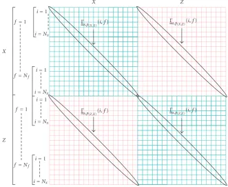
Figure2: Diagram ofΓs,p, the 2-Component wideband spectral matrix of the wavep.
each separated wavefield. State of polarization analysis is based on the computation of parameters describing the particle movement associated with wave propagation. That movement of the ground induced useful parameters which were first identified by Jolly in 1956 [27], whereas the first attempt to measure this movement was done by Shimshoni and Smith in 1964 [28]. They introduced a successful method of polarization analysis for earthquake data. Many other algorithms were developed subsequently for seismic exploration applications [29–31]. One of the most effective and stable approaches in this regards is the algorithm developed by Flinn [32,33] using the covariance matrix of the data. In the following part, we compare our proposed method (based on MWSM) with Flinn’s algorithm.
3.2. Proposed Method. We propose to use the spectral matrices of rank one (linked to each pth source) obtained from the decomposition of the multicomponent wideband spectral matrix (see (15)). Thus, once a wavefield has been separated from other waves and from noise, we show that its polarization parameters can be characterized from the matrix elements of wavefield, Γs,p. After separation processing, the signal, notedOx,p,i(f), corresponding to the
pth source received on componentXat frequency f and on sensorican be expressed as
Ox,p,i
f=apwp
fe−j2π f τi(θp), (18)
whereτi(θp) is the time of propagation between the source
and the sensori(for wavep). For the second componentZ,
we obtain
Oz,p,i
f=αpejϕpapwp
fe−2jπ f τi(θp). (19)
The diagonal element of Γs,p at the frequency f on the
ith sensor which corresponds to the interaction of the X
component with itself could be expressed by
Γs,p
(X,X)
i,f=σ2
pwp
f2. (20)
Likewise, the term corresponding to the interaction of Z component with itself is
Γs,p
(Z,Z)
i,f=α2
pσp2wp
f2 (21)
and finally, the cross-term corresponding to the interaction between componentXandZcould be written as
Γs,p
(X,Z)
i,f=αpσ2pwp
f2e−jϕp. (22)
All these terms are located either on the principal diagonal or on the secondary diagonals of the matrix Γs,p (see
Figure 2). Based on these structures, we deduce estimators for polarization parameters of the pth wave on each sensor
0 0.1 0.2 0.3 0.4 0.5 0.6 0.7 0.8
−10 −5 0 5 10 15
MAE
SNR (dB) Proposed method
Flinn’s method
Figure 3: Mean Absolute Error for estimation of phase shift
between components for various SNRs (plain line: MWSM based method; dotted line: Flinn’s method).
expressed as amplitude ratio between componentsXandZ
and phase shift for wavepcan be expressed, respectively, by
αp(X,Z)
i,f=
Γs,p(Z,Z)
i,f
Γs,p
(X,X)
i,f,
ϕp(X,Z)
i,f=arg Γs,p(X,Z)i,f.
(23)
Classically, the propagation medium is regarded as isotropic (nondispersive for frequency) so that the polariza-tion parameters are independent of frequency and sensor. But in more realistic context where some dispersion appears, a better estimate of the polarization parameters can thus be obtained by averaging them over a range of frequencies and sensors. However, in order to have a correct estimate, the averaging must be done only on the frequencies belonging to the signal bandwidth (L3dB=[finf,fsup]). The estimators thus obtained are
αp(X,Z)=
1
card(L3 dB)·Nx Nx
i=1
fsup
f=finf
Γs,p
(Z,Z)
i,f
Γs,p
(X,X)
i,f, (24)
ϕp(X,Z)=arg
⎡
⎣ 1
card(L3 dB)·Nx Nx
i=1
fsup
f=finf
Γs,p
(X,Z)
i,f
⎤ ⎦ (25)
with card(L3 dB) being the cardinal ofL3 dB.
3.3. Comparison between Flinn’s Method and Proposed Method
Based on MWSM. MWSM’s and Flinn’s methods are two
different approaches for polarization analysis. Flinn’s method uses a covariance matrix and proposes a temporal approach on a single trace whereas our proposed method is a frequential approach which can either be on a single trace or on the whole array. In the case studied here, the waves’
0 0.05 0.1 0.15 0.2 0.25 0.3 0.35 0.4 0.45 0.5
−10 −5 0 5 10 15
MAE
SNR (dB) Proposed method
Flinn’s method
Figure 4: Mean Absolute Error for estimation of the amplitude
ratio between components for various SNRs (plain line: MWSM based method; dotted line: Flinn’s method).
state of polarization can be considered as constant over distance. Consequently, for a given wave, we can estimate the amplitude ratio and phase shift between the components by carrying out an averaging of the parameters found on each sensor.
To compare Flinn’s and our method and to illustrate polarization estimation, we consider the trivial case of a single wave with infinite velocity, received on a 2C-sensors array, whose phase shiftϕ(=0.4 rad) and amplitude ratioα
(=0.8) are constant over the array.
Figures 3 and 4 correspond respectively to the Mean Absolute Error (MAE) between the theoretical and the estimated values of phase shift and amplitude ratio for various signal-to-noise ratio (SNR) from−10 dB to 15 dB. The average is done for 500 noisy realizations.
These figures show that for both methods, polarization analysis is very sensitive to noise and thus the estimates are better when SNR increases. We can notice that our MWSM-based method always gives better estimation than the Flinn’s method for small SNR.
4. Direction-of-Arrival Estimation
10−5 10−4 10−3 10−2
−18 −16 −14 −12 −10 −8 −6 −4 −2 0
MSE
SNR (dB) MCWB-MUSIC
MUSIC LV-MUSIC
Figure 5: Comparison of DOA estimation error for various
methods. (dotted line: Classical MUSIC; semidotted line: LV-MUSIC; plain line: MW-MUSIC).
We define two matricesUs(NxNfNc×P size) andUn
(NxNfNc×(NxNfNc−P) size), containing the eigenvectors
corresponding to signal subspace and noise subspace, respec-tively,
Us=u1,. . .,uP
,
Un=uP+1,. . .,uNxNfNc
.
(26)
These complex matrices enable us to write MWSM as
Γ=UsΛsUHs +σb2UnU
H
n (27)
with Λs being a diagonal matrix containing the P highest eigenvalues. If we multiply (12) on the right byUn, we obtain
ΓUn=SΓASHUn+σb2Un. (28)
By combining (27) and (28) and by using the orthogo-nality property of the matricesUsandUn, we obtain
σ2
bUn=SΓAS
HU
n+σ
2
bUn (29)
which implies:
SHUn=0. (30) We can rewrite it as
SHp UnUHn Sp=0 (31)
with Sp, being the propagation vector corresponding to
the wave p. Thereafter, we note Πn = UnUHn, the matrix corresponding to the projection on noise subspace.
According to relation (31), propagation vectors are orthogonal to noise subspace. Consequently, their projection onΠnis zero. MW-MUSIC algorithm exploits this idea by
5
10
15
20
0 20 40 60 80 100 120 Time
Se
nso
rs
ComponentX
(a)
5
10
15
20
0 20 40 60 80 100 120 Time
Se
nso
rs
ComponentZ
(b)
Figure6: 2-Component initial dataset in time and distance ((a):
Horizontal componentX, (b): Vertical componentZ).
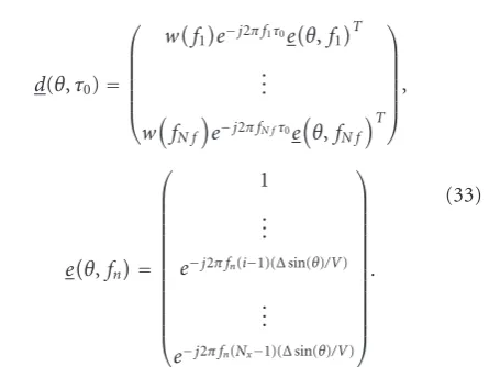
carrying out the projection of directional vectorh(θ,τ0,α,ϕ) on the estimated noise subspace. This vector models the arrival of a polarized wave of directionθon multicomponent sensors’ antenna and is expressed as
hθ,τ0,α,ϕ= 1
NxNfNc
d(θ,τ0)
αejϕd(θ,τ0)
500 1000 1500 2000 2500 3000 200 400 600 800 1000 1200 1400 (1) (2) (3) (4)
500 1000 1500 2000 2500 3000
Figure 7: Modulus of the Multicomponent Wideband Spectral
Matrix of the initial dataset (of size 3072×3072 with 3072 = 24×64×2). Compared withFigure 1, block 1 isΓXX, block 4 is ΓZZand blocks 2 and 3 areΓXZ,ΓZX, respectively.
500 1000 1500 2000 2500 3000
0.5 1 1.5 2 2.5 3 3.5 4 4.5
(1) (2)
(3) (4)
500 1000 1500 2000 2500 3000
×10−3
Figure 8: Modulus of the multicomponent wideband spectral
matrix of the first extracted wave,Γs,1.
with
d(θ,τ0)=
⎛ ⎜ ⎜ ⎜ ⎜ ⎜ ⎝
wf1e−j2π f1τ0eθ,f1T
.. .
wfN f
e−j2π fN fτ0e
θ,fN f
T ⎞ ⎟ ⎟ ⎟ ⎟ ⎟ ⎠,
eθ,fn
= ⎛ ⎜ ⎜ ⎜ ⎜ ⎜ ⎜ ⎜ ⎜ ⎜ ⎜ ⎜ ⎜ ⎝ 1 .. .
e−j2π fn(i−1)(Δsin(θ)/V)
.. .
e−j2π fn(Nx−1)(Δsin(θ)/V)
⎞ ⎟ ⎟ ⎟ ⎟ ⎟ ⎟ ⎟ ⎟ ⎟ ⎟ ⎟ ⎟ ⎠ . (33) 500 1000 1500 2000 2500 3000 1 2 3 4 5 6 7 8 9 (1) (2) (3) (4)
500 1000 1500 2000 2500 3000
×10−3
Figure 9: Modulus of the multicomponent wideband spectral
matrix of the second extracted waveΓs,2.
The extended MUSIC functional, calculated by projec-tion ofh(θ,τ0,α,ϕ) on the noise subspace is given by
MW−MUSICθ,τ0,α,ϕ
= 1
hθ,τ0,α,ϕH Πnhθ,τ0,α,ϕ.
(34)
The functional allows local maxima for a set of valuesθ,τ0,α, andϕ. We use the fact that two parameters (α,ϕ) have been already found by the method proposed on Section 3. After this stage, the functional only depends on two parameters,
θ the direction of arrival andτ0, the offset, and it will give maximum for values of (θ,τ0) corresponding to the sources present in the signal. It is clear that processing will work with lot of efficiency in case of far field sources (waves can be considered as locally plane).
4.2. Study of Estimator Variance. In this part, we compare variances of various estimators: MUSIC, LV-MUSIC and MW-MUSIC. Mean Square Error (MSE) for DOA estima-tion is presented for various SNRs (Figure 5). Each point corresponds to an average over 200 realizations. In this case under study, a polarized source is received on an array of 30 2C-sensors. The DOA of the source, expressed in terms of samples of delay between two sensors, is 1 sample. A white Gaussian noise is added to the signal with a SNR from−18 dB to 0 dB. For classical MUSIC algorithm which operates only on one component, we carry out an average of the results obtained from the two components.
5
10
15
20
0 20 40 60 80 100 120 Time
Se
nso
rs
ComponentX
(a)
5
10
15
20
0 20 40 60 80 100 120 Time
Se
nso
rs
ComponentZ
(b)
Figure10: First extracted wave after projection of initial dataset
onto the first eigenvector. (a) ComponentX, (b) ComponentZ.
5. Synthetic Examples
Proposed method consisting of wavefield separation followed by polarization and DOA estimation steps is applied on a 2-Components synthetic seismic profile to validate the efficiency of the method.Figure 6plots two waves received on an array of 24 2C-sensors superimposed by a white gaussian noise (SNR=4 dB). The fastest wave, (calledwave 1) has a linear polarization parameter (α=1.5 andϕ=0 rad)
5
10
15
20
0 20 40 60 80 100 120 Time
Se
nso
rs
ComponentX
(a)
5
10
15
20
0 20 40 60 80 100 120 Time
Se
nso
rs
ComponentZ
(b)
Figure11: Second extracted wave after projecting initial dataset on
the second eigenvector. (a) ComponentX, (b) ComponentZ.
and the slowest wave (calledwave 2) is characterized by an elliptic polarization (α=1.5 andϕ=1.5 rad).
1 2 3 4 5
500 1000 1500 2000 2500 3000 ×10−3
(1) (4)
(3) (2)
500 1000 1500 2000 2500 3000 2
0 −2
Figure12: Upper plot=modulus of diagonals of blocks (1) and (4)
diagonals of the spectral matrix ofwave 1(Figure 8). Bottom plot: angle of blocks (2) and (3) diagonals of the spectral matrix ofwave 1(Figure 8).
−0.5 −1−1.5
−2−2.5 −3 0 20 40 60 80 100 120 0
2 4 6 8 10 12
Offset DOA (pts.)
×104
Figure13: Amplitude of MW-MUSIC functional as a function of
DOA and offset.
is presented in Figure 7. We observe the same structure as in Figure 1 where the large energetic pattern is associated to wave 1 (low frequency content), and smaller energetic pattern to wave 2 (high frequency content). The MWS Matrix is then decomposed using eigenvalue decomposition. Observing the decrease of eigenvalues, we decide to keep the two first eigen sections, corresponding to modeled waves:
Γs,1=λ1u1uH1, Γs,2=λ2u2uH2. (35)
Figures8and9show the modulus ofΓs,1(wave 1) andΓs,2
(wave 2). We can observe from these figures that separation of waves is efficient since patterns are well separated and no energetic interferences appear. Thus, by projecting the initial data on the first eigenvector u1, we obtain the first extracted wavefield (wave 1) (Figure 10) and on the second eigenvector u2, the second extracted wavefield (wave 2)
(Figure 11). These two figures clearly show that the noise has been removed and the waves have been well separated.
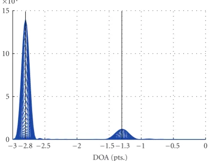
0 5 10 15 ×104
−3−2.8−2.5 −2 −1.5−1.3 −1 −0.5 0 DOA (pts.)
Figure14: DOA estimation (cross-section for various offsets).
Table1: True and estimated values of polarization parameters of
wave 1andwave 2.
True values Estimated values
wave 1 α1=1.5 "α1=1.1
ϕ1=0 rad ϕ"1=3·10−2rad
wave 2 α2=1.5 α"2=1.17
ϕ2=1.5 rad "ϕ2=1.54 rad
5.2. Polarization Estimation. After separation of waves, the second step consists of making the polarization analysis of the two waves using the matrix elements of Γs,1 and
Γs,2 (see Section 3). As previously presented, in Figure 8
(resp.,Figure 9), blocks (1) and (4) correspond to wideband spectral matrices ofwave 1(resp.,wave 2) on components
XandZ, respectively. We denote them byΓs,1(X,X)andΓs,1(Z,Z)
(resp., Γs,2
(X,X) and Γs,2(Z,Z)). Blocks (2) and (3) correspond
to the cross-spectral matrices of wave 1 (resp., wave 2) containing the interactions between componentsX andZ.
We denote them by Γs,1(X,Z) and Γs,1(Z,X) (resp., Γs,2(X,Z) and
Γs,2
(Z,X)).
Figure 12shows two graphs. The upper plot corresponds to the modulus of diagonals of blocks (1) and (4) ofΓs,1. It enables to determine the frequency bandL1=[finf 1,fsup 1] used to estimate the polarization parameters as well as to carry out the estimation of the amplitude ratioα1"between components X and Z (see (25)). The bottom graph of
Figure 12shows the phase of blocks (2) and (3) diagonals. It allows to obtain phase shiftϕ1"between componentsXand
Z (see (25)). In a similar way, it is possible to estimate the polarization parameters ofwave 2by using the principal and secondary diagonals of the spectral matrixΓs,2.
The values obtained for the polarization parameters of each wave are summarized in Table 1. The phase shift ϕ
0
5
10
15
20
25
30
0 20 40 60 80 100
Temps
Cap
teurs
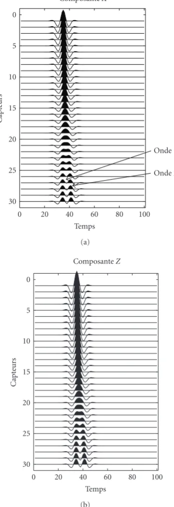
Onde 1 Onde 2 ComposanteX
(a)
0
5
10
15
20
25
30
0 20 40 60 80 100
Temps
Cap
teurs
ComposanteZ
(b)
Figure15: Model of two waves with close DOAs.
to estimate MWSM might affect the wave amplitudes since smoothing is equivalent to an averaging in distance over a small number of sensors.
5.3. DOA Estimation. The last step is the estimation of DOA and offset of each wave (seeSection 4). We compute the MW-MUSIC functional for values of the DOA, ξ(θ), between [−3; 3] with a step of 0.01 and for the offset
τ0, between [0; 127] with a step of 1. The results obtained are shown in Figure 13. The two main lobes are found at
0
5
10
15
20
25
30
0 20 40 60 80 100
Temps
Cap
teurs
ComposanteX
(a)
0
5
10
15
20
25
30
0 20 40 60 80 100
Temps
Cap
teurs
ComposanteZ
(b)
Figure16: Initial noisy dataset.
the original values of offsets and DOAs of the two waves samples.Figure 14corresponds to the cross-sections of the 3D-function (Figure 13) for fixed offsets. The vertical lines show the theoretical values of the DOAs. The estimated values for the DOAs and the offsets are recapitulated in
Table 2. One can note that the estimated values are very close to the true values (percentages of error between 0 and 4%).
0 0.1 0.2 0.3 0.4 0.5 0.6 0.7 0.8 0.9 1
−2 −1.5 −1 −0.5 0 0.5 1 1.5 2 DOA en echantillons
MCWB-MUSIC LV-MUSIC
−0.2
Figure17: Comparison between MW-MUSIC and LV-MUSIC.
Table2: Estimation of DOAs and offsets.
DOA (pts.) Offset (pts.)
True Values Estimated Values True Values Estimated Values
wave 1 −1.3 −1.30 28 27
wave 2 −2.8 −2.84 44 42
These two waves calledOnde1 andOnde2 have shown same spectrum, same offset, same polarisation parameters, and two very close DOAs (ξ(θO1) = 0; ξ(θO2) = −0.2). The
Signal-to-Noise ratio is estimated at 0 dB (Figure 16). We propose to compare Long Vector-MUSIC and Multi-component Wideband-MUSIC algorithms. We show on
Figure 17, that resolution given by MW-MUSIC is better than LV-MUSIC. A full separation, polarisation and DOA’s estimation have been also realized on a real seismic example [41].
6. Conclusion
A novel method providing wavefields separation along with an estimation of both the polarization parameters and the directions of arrival was presented. Taking into account the polarization and the widebandness of the signal leads to a better characterization of a greater number of waves (NxNfNc−1) as opposed to the monocomponent array case
(Nx −1). The performance and efficiency of the method
was proven using several simulations. Comparison of the wideband matrix filtering method with those of the classic filtering technique has already been done [15] and gave encouraging result for wideband case. We also obtained promising results for DAO estimation using the proposed method which can be attributed to the fact that our method takes into account the entire frequency information and is therefore insensitive to frequency band selection.
Acknowledgments
The authors would like to thank reviewers for interesting remarks and A. A. Khan for improving the language.
References
[1] A. Nehorai and E. Paldi, “Vector-sensor array processing for electromagnetic source localization,” IEEE Transactions on Signal Processing, vol. 42, no. 2, pp. 376–398, 1994.
[2] A. Nehorai and E. Paldi, “Acoustic vector-sensor array process-ing,”IEEE Transactions on Signal Processing, vol. 42, no. 9, pp. 2487–2491, 1994.
[3] J. Li and R. T. Compton Jr., “Angle and polarization estimation using ESPRIT with a polarization sensitive array,” IEEE Transactions on Antennas and Propagation, vol. 39, no. 9, pp. 1376–1383, 1991.
[4] D. Rahamim, J. Tabrikian, and R. Shavit, “Source localization using vector sensor array in a multipath environment,”IEEE Transactions on Signal Processing, vol. 52, no. 11, pp. 3096– 3103, 2004.
[5] H.-W. Chen and J.-W. Zhao, “Wideband MVDR beamforming for acoustic vector sensor linear array,”IEE Proceedings: Radar, Sonar and Navigation, vol. 151, no. 3, pp. 158–162, 2004. [6] K. T. Wong and M. D. Zoltowski, “Self-initiating
MUSIC-based direction finding and polarization estimation in spatio-polarizational beamspace,”IEEE Transactions on Antennas and Propagation, vol. 48, no. 8, pp. 1235–1245, 2000.
[7] K. T. Wong and M. D. Zoltowski, “Diversely polarized root-MUSIC for azimuth-elevation angle-of-arrival estimation,” inProceedings of the AP-S International Symposium & URSI Radio Science Meeting, pp. 1352–1355, July 1996.
[8] K. T. Wong and M. D. Zoltowski, “Root-MUSIC-based azimuth-elevation angle-of-arrival estimation with uniformly spaced but arbitrarily oriented velocity hydrophones,”IEEE Transactions on Signal Processing, vol. 47, no. 12, pp. 3250– 3260, 1999.
[9] K. T. Wong and M. D. Zoltowski, “Uni-vector-sensor ESPRIT for multisource azimuth, elevation, and polarization estima-tion,”IEEE Transactions on Antennas and Propagation, vol. 45, no. 10, pp. 1467–1474, 1997.
[10] M. D. Zoltowski and K. T. Wong, “Closed-form eigenstructure-based direction finding using arbitrary but identical subarrays on a sparse uniform Cartesian array grid,”IEEE Transactions on Signal Processing, vol. 48, no. 8, pp. 2205–2210, 2000.
[11] M. D. Zoltowski and K. T. Wong, “ESPRIT-based 2-D direc-tion finding with a sparse uniform array of electromagnetic vector sensors,”IEEE Transactions on Signal Processing, vol. 48, no. 8, pp. 2195–2204, 2000.
[12] K. T. Wong and M. D. Zoltowski, “Closed-form direction finding and polarization estimation with arbitrarily spaced electromagnetic vector-sensors at unknown locations,”IEEE Transactions on Antennas and Propagation, vol. 48, no. 5, pp. 671–681, 2000.
[13] K. T. Wong, L. Li, and M. D. Zoltowski, “Root-MUSIC-based direction-finding and polarization estimation using diversely polarized possibly collocated antennas,”IEEE Antennas and Wireless Propagation Letters, vol. 3, no. 1, pp. 129–132, 2004. [14] C. Paulus, J. Mars, and P. Gounon, “Wideband spectral matrix
filtering for multicomponent sensors array,”Signal Processing, vol. 85, no. 9, pp. 1723–1743, 2005.
[15] C. Paulus and J. I. Mars, “New multicomponent filters for geophysical data processing,”IEEE Transactions on Geoscience and Remote Sensing, vol. 44, no. 8, pp. 2260–2270, 2006. [16] H. Mermoz, “Imagerie, corr´elation et mod`eles,”Annales des
[17] J. C. Samson, “The spectral matrix, eigenvalues, and principal components in the analysis of multichannel geophysical data,”
Annales Geophysicae, vol. 1, no. 2, pp. 115–119, 1983. [18] E. A. Robinson, “Predictive decomposition of time series with
application to seismic exploration,”Geophysics, vol. 32, pp. 418–484, 1967.
[19] B. D. Rao and K. V. S. Hari, “Weighted subspace methods and spatial smoothing. Analysis and comparison,” IEEE Transactions on Signal Processing, vol. 41, no. 2, pp. 788–803, 1993.
[20] S. S. Reddi, “On a spatial smoothing technique for multiple source location,”IEEE Transactions on Acoustics, Speech, and Signal Processing, vol. 35, no. 5, p. 709, 1987.
[21] T. Shan, M. Wax, and T. Kailath, “On spatial smoothing for direction-of-arrival estimation of coherent signals,”IEEE Transactions on Acoustics, Speech, and Signal Processing, vol. 33, no. 4, pp. 806–811, 1985.
[22] S. U. Pillai and B. H. Kwon, “Forward/backward spatial smoothing techniques for coherent signal identification,”IEEE Transactions on Acoustics, Speech, and Signal Processing, vol. 37, no. 1, pp. 8–15, 1989.
[23] H. Wang and M. Kaveh, “Coherent signal-subspace processing for the detection and estimation of angles of arrival of multiple wide-band sources,” IEEE Transactions on Acoustics, Speech, and Signal Processing, vol. 33, no. 4, pp. 823–831, 1985. [24] N. Thirion, J. I. Mars, and J.-L. Lacoume, “Analytical links
between steering vectors and eigenvectors,” inProceedings of the European Signal Processing Conference (EUSIPCO ’96), pp. 81–84, Trieste, Italy, 1996.
[25] N. Thirion, J. Lacoume, and J. Mars, “Resolving power of spectral matrix filtering: a discussion on the links steering vectors / eigenvectors,” inProceedings of the 8th IEEE Signal Processing Workshop on Statistical Signal and Array Processing (SSAP ’96), pp. 340–343, June 1996.
[26] N. Thirion, J. I. Mars, and J.-L. Boelle, “Separation of seismic signals: a new concept based on blind algorithm,” in Proceedings of the European Signal Processing Conference (EUSIPCO ’96), pp. 85–88, Trieste, Italy, 1996.
[27] R. N. Jolly, “Investigation of shear waves,”Geophysics, vol. 21, no. 4, pp. 905–938, 1956.
[28] M. Shimshoni and S. W. Smith, “Linear end parabolic τ-p revisited,”Geophysics, vol. 29, no. 5, pp. 664–671, 1964. [29] S. A. Greenhalgh, I. M. Mason, C. C. Mosher, and E.
Lucas, “Seismic wavefield separation by multicomponent tau-p tau-polarisation filtering,”Tectonophysics, vol. 173, no. 1-4, pp. 53–61, 1990.
[30] C.-S. Shieh and R. B. Herrmann, “Ground roll: rejection using polarization filters,”Geophysics, vol. 55, no. 9, pp. 1216–1222, 1990.
[31] G. M. Jackson, I. M. Mason, and S. A. Greenhalgh, “Principal component transforms of triaxial recordings by singular value decomposition,”Geophysics, vol. 56, no. 4, pp. 528–533, 1991. [32] E. A. Flinn, “Signal analysis using rectilinearity and direction of particule motion,”Proceedings of the IEEE, vol. 56, pp. 1874– 1876, 1965.
[33] C. B. Archambeau and E. A. Flinn, “Automated analysis of seismic radiation for source characteristics,”Proceedings of the IEEE, vol. 53, pp. 1876–1884, 1965.
[34] R. O. Schmidt,A signal subspace approach to multiple emitter location and spectral estimation, Ph.D. dissertation, Stanford University, Stanford, Calif, USA, 1981.
[35] R. O. Schmidt, “Multiple emitter location and signal param-eter estimation,”IEEE Transactions on Antennas and Propaga-tion, vol. 34, no. 3, pp. 276–280, 1986.
[36] M. Kaveh and A. J. Barabell, “The statistical performance of the MUSIC and the minimum-norm algorithms in resolving plane waves in noise,”IEEE Transactions on Acoustics, Speech, and Signal Processing, vol. 34, no. 2, pp. 331–341, 1986. [37] P. Stoica and A. Nehorai, “MUSIC, maximum likelihood, and
Cramer-Rao bound,”IEEE Transactions on Acoustics, Speech, and Signal Processing, vol. 37, no. 5, pp. 720–741, 1989. [38] E. R. Ferrara Jr. and T. M. Parks, “Direction finding with
an array of antennas having diverse polarizations,” IEEE Transactions on Antennas and Propagation, vol. 31, no. 2, pp. 231–236, 1983.
[39] Y. Hua, “Pencil-MUSIC algorithm for finding two-dimensional angles and polarizations using crossed dipoles,”
IEEE Transactions on Antennas and Propagation, vol. 41, no. 3, pp. 370–376, 1993.
[40] A. Swindlehurst and M. Viberg, “Subspace fitting with diversely polarized antenna arrays,” IEEE Transactions on Antennas and Propagation, vol. 41, no. 12, pp. 1687–1694, 1993.