Article
1
Development of a pattern recognition methodology
2
with thermography and implementation in an
3
experimental study of a boiler for a WHRS-ORC
4
Concepción Paz 1,*, Eduardo Suárez 1, Miguel Concheiro 1 and Antonio Diaz 1
5
1 School of Industrial Engineering, University of Vigo, Campus Universitario Lagoas-Marcosende, 36310,
6
Spain; [email protected] (E.S.); [email protected] (M.C.); [email protected] (A.D.)
7
* Correspondence: [email protected]; Tel.: +34 986 813 754
8
9
Abstract: Waste heat dissipated in the exhaust system in a combustion engine represents a major
10
source of energy to be recovered and converted into useful work. A waste heat recovery system
11
(WHRS) based on an Organic Rankine Cycle (ORC) is a promising approach, and has gained interest
12
in the last few years in an automotive industry interested in reducing fuel consumption and exhaust
13
emissions. Understanding the thermodynamic response of the boiler employed in an ORC plays an
14
important role in steam cycle performance prediction and control system design. The aim of this
15
study is therefore to present a methodology to study these devices by means of pattern recognition
16
with infrared thermography. In addition, the experimental test bench and its operating conditions
17
are described. The methodology proposed identifies the wall coordinates, traces paths, and tracks
18
wall temperature along them in a way that can be exported for subsequent post-processing and
19
analysis. As for the results, through the wall temperature paths on both sides (exhaust gas and
20
working fluid) it was possible to quantitatively estimate the temperature evolution along the boiler
21
and, in particular, the beginning and end of evaporation.
22
Keywords: WHRS; ORC; boiler; infrared thermography.
23
24
1. Introduction
25
Increasingly restrictive international regulations concerning greenhouse gas emissions demand
26
the development of cleaner and more efficient internal combustion engines (ICEs). Most modern
27
diesel engines are achieving a maximum of about 35% in thermal efficiency—the remaining heat is
28
simply wasted. Waste heat is dissipated through three main channels: the coolant system, convection
29
and radiation from the engine block, and—most importantly—the exhaust system, which alone
30
accounts for up to 40% of total fuel energy [1–4].
31
In the last few years, the automotive industry has shown great interest in waste heat recovery
32
systems (WHRS) based on an Organic Rankine Cycle (ORC) because of its potential for recovering
33
some of that energy. This would achieve significant reductions in fuel consumption and, as a result,
34
exhaust emissions [4–6]. This technology has already been widely implemented over the past decade
35
in the marine sector [7-8], but reducing the components of the cycle to the scale of a passenger vehicle
36
is still a challenge. Nevertheless, there is room to work with in heavy duty vehicles, and so work has
37
continued[9].
38
Predicting the behavior of a boiler is fundamental in the development and design process of
39
these systems. Most boiler load losses are due to the superheated steam zone, so it is very important
40
to estimate its length adequately. In principle, there are correlations that can be used to predict a
41
boiler’s thermal efficiency and head loss. These correlations are different for each section, though, so
42
determining the location of phase changes in a boiler is essential.
43
This study sets out to do just that using a test bench with an ORC-WHRS boiler. We study it
44
from two different approaches: on one hand, the monitored sensors retrieve overall parameters of
45
the boiler, such as outlet temperature, pressure drop, and performance; on the other hand, an infrared
46
(IR) thermographic camera captures thermal images of the external walls of the boiler.
47
IR thermography is a non-contact and non-destructive technique well consolidated and applied
48
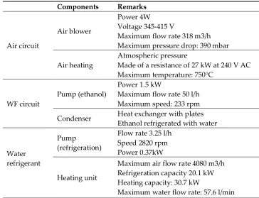
in a wide range of fields, such as medicine and the military [10]. There is even some existing research
49
in the literature that studies multiphase heat transfer processes with thermographic analysis. Liu and
50
Pan [11] developed a method to measure the fluid temperature in parallel with the visualization of
51
the two-phase flow pattern in micro channels. Hetsroni et al. [12] use an IR technique to investigate
52
a heat sink for electronics cooling at low heat fluxes and to maintain the temperature of the heated
53
surface at uniform temperatures. Xu et al. [13] carried out boiling heat transfer experiments where an
54
IR high-speed camera was used to measure a chip’s surface temperature and identify transient flow
55
patterns in an array of triangular silicon-based microchannels. Li and Hrnjak [14] presented an IR
56
thermography-based method to quantify the distribution of liquid refrigerant mass flow rate in a
57
parallel flow microchannel heat exchanger. Leblay et al. [15] measured heat transfer coefficients of
58
water flowing in a round tube and in a multiport flat tube. Carlomagno et al. [16] analyzed the ability
59
of IR thermography to perform convective heat transfer measurements and surface visualizations in
60
complex fluid flows.
61
In the present study, IR thermography has been used to experimentally analyse single phase and
62
multiphase flows involved in the boiler of an ORC. Although the working fluid (WF) is not optically
63
accessible, thermography allows us to quantitatively estimate and understand the fluid dynamic
64
behaviour development of both the gas and the working fluid by inferring their properties from the
65
wall temperatures of their adjacent walls. This study is focused on the implementation of a
66
methodology capable of systematically handling a big database of these thermal images, based on a
67
pattern recognition scheme, which automatically detects the boiler and extracts the temperatures to
68
be analysed.
69
The rest of this paper is divided in three sections. Section 2 describes the experimental setup and
70
the boiler of study. Section 3 presents the methodology developed. Section 4 shows and discusses the
71
results obtained, our conclusions, and an overview of future work.
72
2. Experimental setup
73
The experimental test bench has been conceived as a tool to test boilers for implementation in
74
an ORC-based WHRS for the automotive industry. The working fluid must have a high critical
75
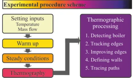
temperature, as well as high condensation and evaporation temperatures, suitable for a
high-76
temperature ORC system. Among the fluids that meet these requirements ─such us ethanol, R1233zd,
77
siloxane, or n-octane─ ethanol was chosen because of its low environmental impact and low health
78
risks [17]. Furthermore, when the facilities were designed, ethanol was the working fluid of choice
79
for many automotive manufacturers.
80
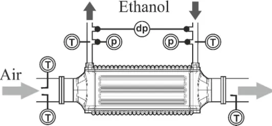
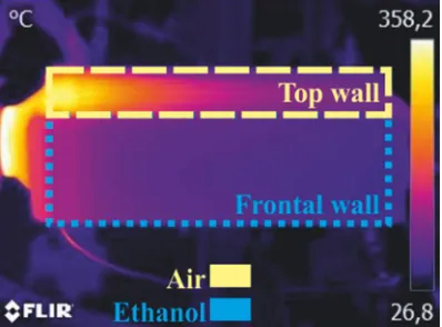
The test bench has three circuits: air, ethanol, and water refrigerant. Ethanol is preheated and
81
pumped to the evaporator, where it comes into contact with previously warmed air. After that, the
82
ethanol is cooled in the condenser by transferring its heat to the refrigeration water. Figure 1 shows
83
85
Figure 1. Schematic diagram of the test bench.
86
The test bench control system is based on a programmable logic controller (PLC). It can be
87
accessed either directly from the test bench or with some complementary software allowing remote
88
access or an SD card suite. Ultimately, the software enables the computer and test bench to exchange
89
information by transferring all the data from the bench to the computer in order to analyse it.
90
The test bench includes a bypass valve system for safe emptying, cleaning and ethanol dragging,
91
in the event the boiler is replaced to test a different one. The characteristics of the main components
92
of the test bench, with the exception of the boiler itself, which is discussed separately in this section,
93
are listed in Table 1.
94
Table 1. Main components of the test bench.
95
Components Remarks
Air circuit
Air blower
Power 4W Voltage 345-415 V
Maximum flow rate 318 m3/h Maximum pressure drop: 390 mbar
Air heating
Atmospheric pressure
Made of a resistance of 27 kW at 240 V AC Maximum temperature: 750°C
WF circuit
Pump (ethanol)
Power 1.5 kW
Maximum flow rate 50 l/h Maximum speed: 233 rpm
Condenser Heat exchanger with plates Ethanol refrigerated with water
Water refrigerant
Pump
(refrigeration)
Flow rate 3.25 l/h Speed 2820 rpm Power 0.37kW
Heating unit
Maximum air flow rate 4080 m3/h Refrigeration capacity 20.1 kW Heating capacity: 30.7 kW
Maximum water flow rate: 57.6 l/min
96
Temperature sensors are distributed all along the test bench to provide the air, ethanol and water
97
temperature at different points of the bench. These points include, among others, the evaporator inlet
98
thermal efficiencies. Pressure drop sensors are mounted on the working fluid side. The main sensors
100
of the experimental setup are described in Table 2.
101
Table 2. Description of the main sensors of the test bench.
102
Sensor Remarks Uncertainty
Air Sensor K 1.5 °C
Water/Ethanol Sensor T 0.5 °C
Pressure drop Differential pressure transducer 0.4% Mass flow rate Coriolis mass flow meter 0.11%
103
The air circuit provides air at a suitable temperature and flow rate to the evaporator after being
104
heated in the heating system. It has three main components: blower, flow rate gauge, and heating
105
system. It basically consists of an open circuit, where air is taken from the environment using an
106
electric turbine as a blower, and a heating system, where the air’s temperature is gradually increased
107
until the required temperature before entering the boiler.
108
The ethanol circuit is the operation control most prone to instabilty in the whole system. It is
109
designed to pump the liquid ethanol into the evaporator and then through a condenser, where it is
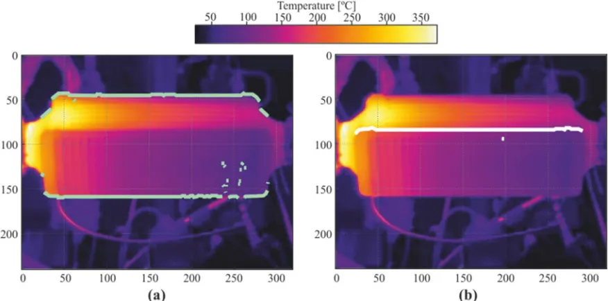
110
cooled before entering a storage tank being pumped again. The eccentric screw pump pumps the
111
ethanol at the set pressure. Just before entering the boiler, an electric preheater helps the ethanol’s
112
temperature to rise to the set temperature. A plate condenser cools the ethanol after the expansion
113
valve. The storage tank stores all the ethanol after it is cooled in the condenser and keeps it at the
114
proper pressure before entering the pump again.
115
The experimental bench also has a refrigeration system that cools the hot ethanol leaving the
116
evaporator and further cools the ethanol before entering the storage tank. The components of this
117
circuit are: a centrifugal pump that pressurizes the water so it reaches the condenser; a regulation
118
valve, and; a heating unit, which consists of a forced convection air heater. The working fluid for this
119
system is water, which flows through the condenser in counter-current.
120
The boiler studied is a shell and tube heat exchanger in cross flow and counter flow, made
121
entirely of steel AISI 316L. Air flows through a bundle of staggered tubes, while the working fluid
122
flows inside them, in a cross-flow configuration. After the working fluid intake, this flow is divided
123
between the first row of tubes, which at the end converge into a mixture chamber to be divided again
124
in the following row. Every mixing chamber only connects one row of tubes with the following one.
125
The performance of the boiler is monitored continuously with thermocouples measuring inlet and
126
outlet air and working fluid temperatures. Pressure drop on both sides are recorded by pressure
127
sensors and a differential pressure sensor. The boiler has been fully coated in thermal black paint on
128
its external surfaces in order to make a visual contrast with the background and avoid shiny
129
reflections in the surface of metal, which could introduce errors in the measurements with the
130
thermographic camera. This black coating increases the emissivity of thermal radiation of the boiler,
131
which according to the specification of the manufacturer is is equal to 0.98, an effect that is taken into
132
account later in the results discussion. Figure 2 represents the boiler studied and Table 3 summarizes
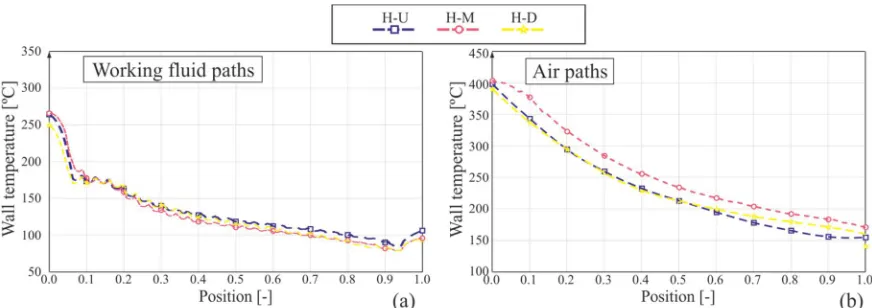
133
its geometrical remarks.
134
135
137
Wall temperature was monitored using the thermographic camera Flir E60, by Flir Systems.
138
Some technical characteristics of the camera are shown in Table 3.
139
Table 3. Main features of the thermographic camera used.
140
Model Flir E60
Range of temperature -20°C to 650°C Thermal sensitivity <0.05° to 30°
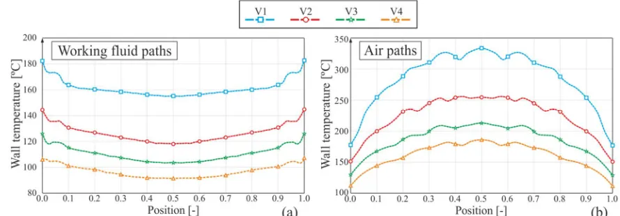
Resolution 320 x 240 pixels
3. Methodology
141
The predominant experimental tool used in this study was infrared thermography. The objective
142
of this noninvasive method was to extract a continuous wall temperature profile along the boiler,
143
which provides information about the fluid underneath the walls. This section is divided in two parts:
144
first, the experimental procedure--that is, how the experiments were carried out and what
145
considerations were taken when the thermal images were shot; and second, the post-processing of
146
the thermal images.
147
3.1. Experimental procedure
148
The experimental procedure is summarized in Figure 3. To run the experiments at the test bench,
149
the inputs of the circuit are set in the bench software: inlet temperature, pressure, and mass flow rate
150
for both air and ethanol circuits. Firstly, the test bench needs to be warmed up. This is done by
151
gradually introducing the desired values of mass flow and system temperature in the both circuits.
152
It is done to ensure a proper functioning and avoid overheating and any damage to the components.
153
The measurements and the thermal images are taken once the monitored outputs confirm that the
154
test has reached a steady state. Subsequent experiments can be performed using the conditions of the
155
previous one, without the need to restart the circuit configuration again.
156
157
Figure 3. Scheme of the experimental procedure.
158
As shown in Figure 4, from the point of view of the thermal image, the top wall is adjacent to
159
the gas side, whereas the frontal wall is adjacent to the mixing chambers of the working fluid, thus
160
the thermographic analysis of these walls makes it possible to quantitatively learn about
161
thermodynamic behaviour of the fluids inside the boiler. Bearing this idea in mind, the relative
162
positioning of the thermographic camera and the boiler makes it possible to picture two walls at a
163
time, one adjacent to the fluid and the other adjacent to the gas. Figure 4 shows a schematic view of
164
the perspective of the boiler from the camera.
165
167
Figure 4. Schematic view of the thermographies.
168
The images were taken by placing the camera on a tripod at a distance of approximately 50 cm
169
at an angle of about 30° relative to the frontal wall. The thermographic camera used, the model Flir
170
E60, takes pictures with a resolution of 320x240 pixels and can measure in a range of temperatures
171
from 0°C to 650°C with an accuracy of ±2°C or ±2% at room temperature and a sensitivity of 0.05°C.
172
3.2. Thermographic processing
173
Raw thermal images were post-processed with the free software Flir Tools. This software can
174
convert the temperature of every pixel into an array of the dimension of the resolution of the camera
175
with the values of temperature in each element. This array is then exported to Matlab in a *.csv file,
176
which performs the calculations needed in this study. The thermal image shows the wall temperature
177
of the boiler, but also the temperatures of the background of the scene. Since these values are not of
178
interest, they were eliminated in the processing.
179
To do this, a very simple method was tested first. The images were given a temperature limit,
180
and all the pixels (in .csv, a cell and in Matlab, an element of the array) that did not reach a minimum
181
temperature had their values converted to NaN. Then, pixels were arranged by rows and by columns,
182
with all rows and columns with an average value of NaN lower than a certain value being eliminated.
183
To eliminate the hot tubes that do not completely disappear after the previous filtrations, a filtering
184
process was carried out by columns and rows with a minimum number of non-NaN. This method
185
was quite effective, but in cases where the boiler is inclined, the cutting section was too horizontal
186
and some data were lost. Another problem is that the perspective was lost, and thus the construction
187
of the lines in their correct position.
188
With this in mind, a new methodology was developed. This methodology detects the boiler
189
through a pattern recognition approach. Wall temperature paths were traced and plotted
190
automatically. Wall temperature values in both gas and working fluid regions, both parallel and
191
perpendicular to the flow of the fluids, were tracked. The whole process can be divided in five steps:
192
detecting the boiler, tracking the edges, improving the edges, tracing the walls, and defining the
193
paths. Figure 4 to Figure 9 included in this section are used to illustrate the methodology, and do not
194
represent any particular experimental point.
195
3.2.1. Detecting the boiler
196
To identify the shape of the boiler, a temperature difference filter was applied, thus taking
197
advantage of the sharp difference between the boiler’s and room temperatures. Some pipes and ducts
198
from the circuit can be seen in the thermal image, but they all belong to the ethanol circuit, whose
199
temperatures are significantly lower than the temperature of the boiler. To filter these out, the first
200
step was to coarsely discard the pixels belonging to the background. To do so, the pixels of
201
temperature below a threshold of 40°C is replaced by black pixels, resulting in an image similar to
202
the displayed in Figure 5-a. Notice that some components of the circuit with higher temperatures
203
To discard the remaining undesired pixels, the rows and columns of pixels with less than a
205
threshold number of blank pixels are filtered and set as blank pixels too. A sample of a resulting
206
image is displayed in Figure 5-b. Note that to apply the method shown here, the boiler was positioned
207
as horizontally as possible from the perspective of the thermographic camera.
208
209
Figure 5. (a) Sample of the core of the boiler detected. (b) Sample of thermography after filtering cold pixels
210
in the background.
211
3.2.2. Tracking the edges
212
As shown in Figure 5-b, the boundaries of the boiler are still not neatly defined. To identify the
213
horizontal edges of the boiler, the highest wall temperature gradient is chosen as the next filter criterion.
214
In Figure 6, a 3D graph of temperatures of the boiler is plotted. Here, it is clear that the maximum
215
temperature gradient corresponds to the outermost edges of the boiler from the perspective of the
216
camera. The edge between the top wall and the frontal wall becomes an inflection point of the
217
temperature profiles. Figure 7 shows the reconstruction of the edges of the boiler using this approach.
218
219
Figure 6. 3D graph of the temperatures identified as belonging to the boiler at this step of the procedure.
220
3.2.3. Improving the edges
222
As shown in Figure 7-a, the pixel cloud representing the horizontal edges obtained in the previous
223
step still shows noise and does not seem to be the straight line we know it ought to be. To convert that
224
point cloud into a straight line, two further steps were taken: filtering outliers and a Hough transform
225
[18–20].
226
The outliers were filtered by their deviation from the median of the vertical location of the pixels,
227
when the pixel is an outlier q with the criterion:
228
< − 1.5
or
> + 1.5
(1)
where Q1 and Q3 are the first and the third quartile respectively and IQR is the interquartile range.
229
Once the outliers were filtered, Figure 7-b, a Hough transform was applied. A Hough transform is
230
a digital image processing technique based on feature recognition. The technique consists of identifying
231
any geometrical instance that can be parametrized, such as straight lines, circumferences or ellipses.
232
This very effectively converted the remaining point clouds representing the edges into a straight line.
233
234
Figure 7. (a) The reconstruction of the outermost edges is represented in the colour green. (b) The
235
reconstruction of the middle edge is represented in the colour white.
236
3.2.4. Defining the walls
237
Because the output of the Hough transform is a line —and not a geometrical segment— to define
238
the frontal and top walls in the images, the vertices of the now-clear edges must be found.
239
There are two issues to solve in this phase. The first is that although the outliers points should have
240
been filtered by the criterion previously discussed, it was observed that some of these points remained
241
because they belonged to the gas boxes. The second issue is found in the particular boiler used in this
242
study. Due to its manufacturing procedure, the plaque that makes up the superior wall is framed into
243
the gas boxes, deforming it slightly.
244
Taking these two considerations into account, the vertices of the edges are determined by finding
245
the first point at more than two pixels’ distances from the line previously found with the Hough
246
transform.
247
Once the horizontal edges on the top and frontal walls are defined (Figure 8-a) the remaining
248
vertical edges are defined by tracing a straight line between the vertices of the horizontal edges, thus
249
251
Figure 8. Walls detected by the developed methodology, (a) main edges detected (b) walls of interest (c)
252
studied paths position.
253
3.2.5. Tracing paths
254
Having defined the four edges that define the walls of interest, the path where the properties of
255
wall temperatures is tracked can be defined. Paths of wall temperature are defined on both the frontal
256
and top walls, longitudinal to the flow of both fluids involved. In terms of percentage of the
257
corresponding edge longitude, every path is at 5% away from the vertical edge, and 20%, 50% and 80%
258
away from the middle edge, as shown on the graph Figure 8-c, and in more detail in Figure 9.
259
260
261
Figure 9. Definition and nomenclature of the paths studied.
262
To retrieve the value of the temperature of the paths, the paths were divided into 200 points and a
263
two-dimensional interpolation was calculated between the two nearest pixels from the image, with the
264
vertical coordinate as a reference. To reduce the oscillations in the values of wall temperature due to
265
the ripples of the external surfaces in the paths of both the gas and working fluid sides, profiles of the
266
horizontal wall temperature paths were smoothed using the robust local regression method with
267
weighted linear least squares and a second-degree polynomial model, which was carried out using
268
MATLAB software.
269
4. Results and discussion
270
Throughout the study, we ran the test under different conditions as a control of the
271
methodology. The result of the test carried out under the operating conditions, detailed in Table 4,
272
Table 4. Boiler operating conditions.
274
Ethanol Dry air
Inlet mass flow [kg/h] 30 70
Inlet temperature [°C] 80 700 Pressure outlet [bar-a] 21 1 Outlet temperature [°C] 275.14 131.44
Performance [%] 85.3
275
Figure 10 shows the thermal image corresponding to the test point previously described.
276
277
278
Figure 10. Thermography of the boiler with the operating conditions described in Table 4.
279
The lines in Figure 11-a represent the horizontal profiles of wall temperature in the wall adjacent
280
to the mixture chambers on the working fluid side. The slopes of the curves clearly show 4 stages.
281
From left to right, the first and hotter stage represents the portion of the wall which is adjacent to the
282
gas side. The second stage of the curve shows a portion where there are not great changes in the slope
283
of the curve—in fact it is almost constant—which indicates a phase change on the working fluid side.
284
In the third stage the slope remains negative, indicating that the working fluid is being cooled down
285
in a monophasic flow. In the last stage, wall temperature increases again, where the wall is again
286
adjacent to the gas side.
287
Figure 11-b shows the horizontal paths of wall temperature on the wall adjacent to the gas side,
288
that is, the top wall. As expected, wall temperature decreases along the boiler, while gas is
289
transferring heat to the working fluid and, to a lesser extent, to the environment by free convection
290
and radiation. Figure 12-b shows the vertical paths on the gas side. Notice the wavy pattern of wall
291
temperature, which is easily identified too in a visual analysis of the thermal image in Figure 10.
292
293
Although the geometry of the boiler is almost symmetric, wall temperature in the vertical paths
295
of Figure 12-a are not as symmetric as would be expected, being seriously displaced in every case.
296
This is likely to be mainly due to the perspective of the camera with regard to the boiler, which is not
297
orthogonal. The position of the camera was a compromise solution between having the most
298
information possible in a single image and making the process of taking the images as automated
299
and standardized as possible, with no need to change the camera or boiler position twice in every
300
experiment.
301
302
Figure 12. Graphs of vertical temperature profile: (a) WF paths and (b) in the air.
303
5. Conclusions
304
In this study an experimental bench was presented to test boilers for an Organic Rankine Cycle
305
in a waste heat recover system, as well as a methodology to detect and analyse them via pattern
306
recognition with thermography. This methodology is able to handle a large amount of thermal
307
images in a database and automatically extract paths of wall temperatures. These paths could be
308
useful for developing correlations that can be used in predictive ─zero-dimensional, one-dimensional
309
or CFD─ models.
310
Once the thermal images are analysed, phase transition on the working fluid side is clearly
311
noticeable, identifiable by a stage where wall temperature remains almost constant, in contrast with
312
the remaining length of the path.
313
Future work will focus on the experimental setup, principally by carrying out further analysis
314
of pressure drop in working fluids, and in the thermographic analysis, mainly by comparing the
315
results obtained with a CFD solution and diving deeper into the working fluid phase transition.
316
Acknowledgments: We gratefully acknowledge BorgWarner Turbo and Emission Systems for providing
317
material and technical support.
318
Conflicts of Interest: The authors declare no conflict of interest.
319
References
320
1. Domingues, A.; Santos, H.; Costa, M. Analysis of vehicle exhaust waste heat recovery potential using a
321
Rankine cycle. Energy. 2013, 49, 71–85. https://doi.org/10.1016/j.energy.2012.11.001
322
2. Park, T.; Teng, H.; Hunter, G.L.; van der Velde, B.; Klaver, J. A Rankine Cycle System for Recovering Waste
323
Heat from HD Diesel Engines - Experimental Results. SAE International. 2011.
https://doi.org/10.4271/2011-324
01-1337
325
3. Wang, E.H.; Zhang, H.G.; Fan, B.Y.; Ouyang, M.G.; Zhao, Y.; Mu, Q.H. Study of working fluid selection of
326
organic Rankine cycle (ORC) for engine waste heat recovery. Energy. 2011, 36, 3406–3418.
327
https://doi.org/10.1016/j.energy.2011.03.041
328
4. Wang, T.; Zhang, Y.; Peng, Z.; Shu, G. A review of researches on thermal exhaust heat recovery with
329
Rankine cycle. Renew. Sust. Energ. Rev. 2011, 15, 2862–2871. https://doi.org/10.1016/j.rser.2011.03.015
330
5. He, M.; Zhang, X.; Zeng, K.; Gao, K. A combined thermodynamic cycle used for waste heat recovery of
331
internal combustion engine. Energy. 2011, 36, 6821–6829. https://doi.org/10.1016/j.energy.2011.10.014
6. Horst, T.A.; Rottengruber, H.S.; Seifert, M.; Ringler, J. Dynamic heat exchanger model for performance
333
prediction and control system design of automotive waste heat recovery systems. Appl. Energ. 2013, 105,
334
293–303. https://doi.org/10.1016/j.apenergy.2012.12.060
335
7. Saleh, B.; Koglbauer, G.; Wendland, M.; Fischer, J. Working fluids for low-temperature organic Rankine
336
cycles. Energy. 2007, 32, 1210–1221. https://doi.org/10.1016/j.energy.2006.07.001
337
8. Schmid, H. Less Emission Through Waste Heat Recovery. In Green Ship Technology Conference, London,
338
U.K., 28-29 April 2004.
339
9. Teng, H. Waste Heat Recovery Concept to Reduce Fuel Consumption and Heat Rejection from a Diesel
340
Engine. In SAE International. 2010. https://doi.org/10.4271/2010-01-1928
341
10. Silva, J.J.D; Maribondo, J.F. Analysis of lubricating oils in shear friction tests using infrared thermography.
342
Infrared Phys. Techn. 2018, 89, 291–298. https://doi.org/10.1016/j.infrared.2018.01.023
343
11. Liu T.L.; Pan, C. Infrared thermography measurement of two-phase boiling flow heat transfer in a
344
microchannel. Appl. Therm. Eng. 2016, 94, 568–578. https://doi.org/10.1016/j.applthermaleng.2015.10.084
345
12. Hetsroni, G.; Mosyak, A.; Segal, Z.; Ziskind, G. A uniform temperature heat sink for cooling of electronic
346
devices. Int. J. Heat Mass Transf. 2002, 45, 3275–3286. https://doi.org/10.1016/S0017-9310(02)00048-0
347
13. Xu, J.L.; Zhang, W.; Wang, Q.W.; Su, Q.C. Flow instability and transient flow patterns inside intercrossed
348
silicon microchannel array in a micro-timescale. Int. J. Multiph. Flow. 2006, 32, 568–592.
349
https://doi.org/10.1016/j.ijmultiphaseflow.2006.02.004
350
14. Li H.; Hrnjak, P. Quantification of liquid refrigerant distribution in parallel flow microchannel heat
351
exchanger using infrared thermography. Appl. Therm. Eng. 2015, 78, 410–418.
352
https://doi.org/10.1016/j.applthermaleng.2015.01.003
353
15. Leblay, P.; Henry, J.F.; Caron, D. Leducq, D.; Bontemps, A.; Fournaison, L. Infrared Thermography applied
354
to measurement of Heat transfer coefficient of water in a pipe heated by Joule effect. In 11th Quantitative
355
InfraRed Thermography, Naples, Italy, Jun 2012.
356
16. Carlomagno, G.M.; Cardone, G. Infrared thermography for convective heat transfer measurements. Exp.
357
Fluids. 2010, 49, 1187–1218. https://doi.org/10.1007/s00348-010-0912-2
358
17. Scaccabarozzi, R.; Tavano, M.; Invernizzi, C.M.; Martelli, E. Comparison of working fluids and cycle
359
optimization for heat recovery ORCs from large internal combustion engines. Energy. 2018, 158. 396–416.
360
https://doi.org/10.1016/j.energy.2018.06.017
361
18. Duda, R.O.; Hart, P.E. Use of the Hough Transformation to Detect Lines and Curves in Pictures. Commun.
362
ACM. 1972, 15, 11–15. http://doi.acm.org/10.1145/361237.361242
363
19. Hough, P.V.C. Method for recognizing complex patterns. U.S. Patent 3, 069 654, 1962.
364
20. Torrente, M.L.; Biasotti, S.; Falcidieno, B. Recognition of feature curves on 3D shapes using an algebraic
365
approach to Hough transforms. Pattern Recogn. 2018, 73, 111–130.
366
https://doi.org/10.1016/j.patcog.2017.08.008