FOR MOBILE POSITIONING IN
CELLULAR COMMUNICATION
Aleksandar Stojcevski
B.E. (Electrical/Electronic)
A thesis submitted in fulfillment of the requirements for the degree of
Master of Engineering
VICTORIA I
UNIVERSITY
H m
« X
z
O
r-o
School of Communications & Informatics
Faculty of Engineering and Science
Victoria University of Technology
Melbourne, Australia
2 £QC=>£ 7 &
r
FTS THESIS 621.38456 STO
30001006983276
I declare that, to the best of m y knowledge, the research described herein is the result of m y o w n work, except where otherwise stated in the text. It is submitted in fulfillment of the candidature for the degree of Masters by Research in Engineering at Victoria University, Australia. N o part of this work has already been submitted for any degree nor is being submitted for any other degree.
Aleksandar Stojcevski
ABSTRACT
In engineering systems there is generally two classes of knowledge: objective knowledge, which can be quantified using the laws of traditional mathematics, and subjective or
intelligent knowledge, that cannot be modeled mathematically but can be expressed in linguistical terms. Fuzzy Logic (FL) is a method that combines these two forms of knowledge, and as such provides a powerful tool for solving real engineering problems.
A fuzzy logic system (FLS) is the methodology of applying FL to engineering systems. In general, a F L S can be considered as a non-linear mapping of crisp (firm) input data to crisp output data. It is the inclusion of subjective knowledge in a F L S that leads to a plethora of mapping possibilities, which m a y not be possible using traditional mathematical modeling techniques. A fuzzy logic system consists of four main elements: fuzzification, rule based, inference engine and deffuzification.
Fuzzy logic has been successfully adopted in many real-world automatic control systems including automobile transmission, subway systems, industrial robots, washing machines, cameras and air-conditioners. In contrast, the utilization of fuzzy logic in mobile communications systems is recent and limited. Understanding general mobile communications is essential in order to go on and develop a mobile positioning application.
The successful applications of Fuzzy Logic Control (FLC) techniques in many areas draw a huge amount of attention to its industrial applications. However, lack of structured methods and tools for design and analysis is preventing this revolutionary controller from playing a more significant role in mobile communications.
RADE STOJCEVSKI
His endless support and encouragement has been a great
TABLE
OF CONTENTS
ACKNOWLEDGMENTS i
LIST OF ABBREVIATIONS ii
LIST OF FIGURES vi
LIST OF TABLES viii
CHAPTER 1:
INTRODUCTION THEORY
1.1 Introduction 1 1.2 Existing Communication Technologies 1
1.3 Mobile Location System 3
1.4 Project Formulation 10 1.4.1 Objectives of the W o r k 10
1.4.2 Methodologies and Techniques 11
1.4.3 Thesis Breakdown 11
CHAPTER 2:
THEORETICAL INTRODUCTION AND LITERATURE REVIEW
2.1 Introduction 13 2.2 Analysis of Handover Algorithms 13
2.3 Signal Strength Model . 14
2.4 Analysis of Positioning Algorithm 16 2.5 Mobile Positioning Distribution 18
2.6 Fuzzy Logic 18
CHAPTER 3:
EXSISTING POSITIONING MODELS
4.2 Positioning Simulator 31 4.2.1 System Simulator 33
4.2.1.1 Structure of the System Simulator 33 4.2.1.2 System Simulator Parameters 35 4.2.1.3 Output from the System Simulator 37
4.2.2 Radio Link Simulator 38
4.2.3 Channel Model 39
CHAPTER 5:
PROPOSED CHANNEL MODEL
5.1 Introduction 4 0 5.2 Modeling Parameters 4 0
5.2.1 Delay Spread 4 0 5.2.2 Correlation of Delay Spread Measurements at Different Base Stations 42
5.2.3 Power Delay Profile Shapes 42 5.2.4 Fading and Angles of Arrival 43 5.3 Channel Model Based on the C O D I T Model 44
5.4 Matching the Delay Spread of the Channel Model to the Delay Spread Model 46
5.5 Unresolved Issues 47 5.6 Definition of the Environments 48
5.7 Base Station Antenna Diversity 49
5.8 G S M Adaptation 51 5.8.1 FIR Filter Implementation 51
5.8.2 Sampling in Time Domain 53
5.8.3 Frequency Hopping 54 5.9 Additional Explanation on the Channel Model 54
5.9.4 Range of Validity 59 5.9.5 Delay Spread vs. Distance-Some Physical Reasons 59
5.10 Matlab Software Package 61
CHAPTER 6:
POSITIONING METHODS
6.1 Introduction 64 6.2 The Up-Link T O A Method 64
6.2.1 T O A Estimation 66 6.2.1.1 The Estimation Problem 66
6.2.1.2 Channel Estimation Algorithm 67 6.2.1.3 Multipath Rejection (ICI-MPR) 68
6.2.2 T O A Simulation Chain 70 6.3 The Enhanced-Observed Time Difference (E-OTD) Method 72
6.3.1 M S Based Location System 72 6.3.2 Benefits and Applications 73 6.3.3 E - O T D Computations 74
6.3.3.1 Cramer-Rao Bound 75
CHAPTER 7:
POSITION CALCULATION AND STATISTICAL EVALUATION
7.1 Introduction 77 7.2 "Average Algorithm" Positioning Method 78
7.3 "More Preferable Solution" Positioning Method 86
CHAPTER 8:
FUZZY LOGIC POSITIONING
9.2 Techniques and Results Comparison 103
9.3 Conclusions 105 9.4 Future W o r k 105
REFERENCES 107
APPENDIX A: System Simulator Matlab files 114
APPENDIX B: Channel Model Matlab files 117
APPENDIX C: System Simulator based on Statistical files (Matlab file) 124
ACKNOWLEDGMENTS
I a m indebted to m a n y people for advice and assistance. First on m y list, m y supervisors Dr. Leonid Reznik and Professor Mike Faulkner. Their support and wisdom will never be forgotten. Thanks also to Dr. Jugdutt Singh, M r . Ranjan Mohapatra, research assistant Melvyn Parrera, and the Mobile Communications & Signal Processing Group at Victoria University for their help.
A special thanks for encorangment goes out to my great friend Mr. Dean Cvetkovic. Thanks also to the Stojcevski family, m y father M r . Rade Stojcevski, Mrs. Vera Stojcevska, Bobby Stojcevski and Filip Stojcevski, for their support, patience and understanding.
F D M A Frequency Division Multiple Access T D M A Time Division Multiple Access C D M A Code Division Multiple Access G S M Global System Mobile
M P S Mobile Positioning System T O A Time of Arrival
A O A Angle of Arrival
T D O A Time Difference of Arrival R F Radio Frequency
G P S Global Positioning System
a Estimated angle of incidence of the propagation wave c Speed of Light
At Difference between the time of arrival signals
X Radio signal wavelength
<j> Arriving electrical phase angle p,sec Micro seconds
m Meters
F C C Federal Communication Commission E911 Emergency nine one one
F M Frequency Modulation A M Amplitude Modulation k m Kilometres F L Fuzzy Logic
F L C Fuzzy Logic Control D S P Digital Signal Processing S N R Signal to Noise Ratio s(t) Received Signal Power
r(t) Fast Fading Component A(n) Discrete Time Signal a Standard Deviation v Velocity of Mobile T Sampling Interval RA(k) Autocorrelation
t Path Delay
L Distance between Base Station and Mobile Station B S Base Station
M S Mobile Station
Xm X coordinate of Mobile
Ym Y coordinate of Mobile
XBs X coordinate of Base Station
Y B S Y coordinate of Base Station A V L Automatic Vehicle Location D Distance between Base Stations SR Rhomboid
C O G Centre of Gravity F M Fuzzy M e a n
W F M Weighted Fuzzy M e a n
F A A H Fuzzy Adaptive-interval and Hysterisis threshold handover A V G Averaging Interval
H Y S Hysterisis Level K2 Propagation Constant
d0 Correlation Distance
Ki Transmitter Power
apdp Average Power Delay Profile C P S Cambridge Positioning Systems R M S Root M e a n Square
Gf Lognormal Fading
C/I Carrier to Interference Ratio
M A T L A B Computing environment for high performance numerical computing and Visualisation
C/N Carrier to Noise Ratio rmse Root M e a n Square Error x Delay Spread
Tw Excess Time Delay
Oi M e a n Angle of Arrival at Mobile L O S Line of Sight
Tm M e a n Delay
9j Angle of Arrival H z Hertz p.s Micro Seconds N L O S N o n Line of Sight
E - O T D Enhanced-Observed Time Difference M L C Mobile Location Centre
D T C D Digital Channel Designation N snapshots
a„ Amplitude of Incoming Waves Tn Delay of Incoming Waves
m Nakagami Parameters CIR Channel Impulse Response C P P Channel Power Profile ICI Incoherent Integration
Eb/N0 Bit Energy to Noise Power Spectral Density
C D F Cumulative Distribution Function
bsv Array containing Base Station coordinates t Time of Arrival (seconds)
T Bit Energy to Noise Power Ratio W i Weighted Average
Wsi Belief Degree based on Signal Strength
Figure 1.1: Location determination by angle of arrival (AOA)
Figure 1.2: Location determination by time distance of arrival (TDOA) Figure 2.1: Arrival times of pilot tones to the Mobiles
Figure 2.2: Position finding by use of hyperbolas Figure 2.3: Area of possible mobile positions Figure 2.4: Handover Process
Figure 2.5: Mobile communications with two base stations A and B Figure 3.1: Circular Distribution
Figure 3.2: The observed and predicted, spread of measurements Figure 3.3: Results from residential area
Figure 4.1: Positioning Simulator Figure 4.2: System Simulator Figure 4.3: Radio Link Simulator
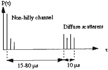
Figure 5.1: The basics of the CODIT channel model
Figure 5.2: Generating the diffuse scatterers for the Hilly channel models of the
CODIT model
Figure 5.3: Model of the local scattering
Figure 5.4: Sample channel for evaluation of the base station angle of arrival model Figure 5.5: Power azimuth spectrum using the model with uniform excess delay
distribution and equal scatterer power (bars), and for a Laplacian
distribution (continuous line). The x-axis is the azimuth angle [deg] and on the y-axis the relative power
Figure 5.6: Phase shifts of waves due to their angle of arrival at the different base
station antennas
Figure 5.7: Plane wave impinging on two spatially separated antennas Figure 5.8: Local scattering
Figure 6.1: GSM transmission chain with time of arrival estimation
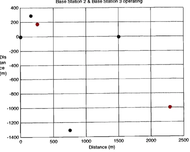
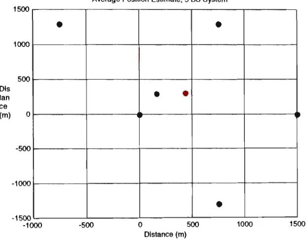
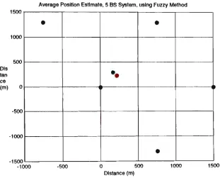
Figure 7.1: Three Base Stations & Original Mobile Station Figure 7.2: Position estimates with BS1 & BS2 operating Figure 7.3: Position estimates with BS1 & BS3 operating Figure 7.4: Position estimates with BS2 and BS3 operating Figure 7.5: Average estimated mobile position for a3BS system Figure 7.6: Average estimated mobile position, for a 5 BS system Figure 7.7: Average estimated mobile position, for a 7 BS system Figure 7.8: Three base station system, Method 2, with BS3 deciding
Figure 7.9: BS1 & BS2 operating, while BS3 makes the decision, 3 BS system Figure 7.10: BS1 & BS3 operating, while BS2 makes the decision, 3 BS system Figure 7.11: BS2 & BS3 operating, while BS1 makes the decision, 3 BS system Figure 7.12: Average position estimate, 5 BS system, using Method 2
Figure 7.13: Average position estimate, 7 BS system, using Method 2 Figure 8.1: Membership function chart.
Figure 8.2: Example of a fuzzy output curve.
Figure 8.3: Base station-Mobile station connections.
Table 2.1: Simulation Parameters
Table 4.1: General parameters to ihe system simulator Table 4.2: Parameters dependent on environment
Table 5.1: Suggested parameter values for the Greenstein delay spread model Table 5.2: Parameters for the CODIT channel model
Table 5.3: Terrain Definitions
Table 8.1: Linguistic meanings of fuzzy logic values. Table 8.2: Membership function
Table 8.3: Fuzzy logic operations.
Table 8.4: Comparison of Boolean Logic and Fuzzy Logic Operations. Table 9.1: Result summary for method 1.
Introduction Theory
CHAPTER 1
INTRODUCTION T H E O R Y
1.1 Introduction
Reliable communications is a virtual component for improvement in performance and increased functionality in mobile location. It provides a very valuable opportunity to present relevant information to the mobile and its occupants. M a n y quality services can be provided to mobiles using communications technologies.
Communications technologies are poised for major expansion in two key areas: wireless data communications and high-speed wireless (wire-based) communications supported by the Internet and ancillary networks. Ultimately it will be the marriage of these two key technologies that will bring about a revolution resulting in a n e w information society. Wireless data applications play a critical role in making the vision of mobile computing a reality. Today's competitive and fast-placed business climate demands tools that allow people to communicate at their o w n convenience and discretion.
1.2 Existing communications technologies
Mobile communications networks need to support m a n y different applications within a wide set of user services including traffic management, emergency management, electronic payment and last but not least mobile location. Each application has specific needs that m a y best be satisfied by a particular communications technology. Because no single communications technology can satisfy all of these requirements, a hybrid implementation of technologies is likely to be required for a regional or statewide communications network.
efficiency, more consistent audio quality throughout more of the coverage area, inherent privacy from analog scanners, and greater data rate capability.
Some of the transmission and switching methods used for transmission of information is briefly considered next. Three major channel access methods exist: F D M A (frequency-division multiple access), T D M A (time-(frequency-division multiple access), and C D M A (code-division multiple access) [1]. F D M A and T D M A can be implemented on either narrowband channels (e.g., 12.5 k H z ) or wideband channels (e.g., 200 kHz), whereas C D M A is restricted to the wideband architecture. T w o principal switching techniques are available: circuit stitching and packet switching. Circuit switching requires the complete end-to-end connection over both the wireless and wired segments before any voice or data can be sent. Packet switching divides the information into packets and transfers packets of data between network nodes over different connections until the packets reach their final destination and are reconstructed for the user. The main difference between these two methods is that circuit switching reserves the required bandwidth in advance, whereas packet switching acquires and releases it on an as-needed bias.
Introduction Theory
trunked radio channel is available. Depending on h o w the available spectrum is used, these systems can also be classified as narrowband or wideband. In the narrow architecture, the total frequency band is split into several narrowband channels. In the wideband architecture, most of the spectrum is available to each and every user.
1.3 Mobile Location Systems
Mobile positioning has received a lot of attention recently. Applications are both of commercial and public interest. Most papers published today illustrate the performance of a mobile positioning technique applicable to the Global System Mobile ( G S M ) network. The ability of a G S M network to locate a mobile station is reduced, for the time being, to the facility required by the mobility management function, i.e. the cell identity. There are s o m e w a y s of improving a rough position of a mobile unit.
O n e of them for example is by using the timing advance information and the management reports. T h e accuracy could be in the order of a few hundred meters. This figure is still not accurate enough for the effective development of a number of n e w added value services and emergency services.
Some of the general questions that arise among us today about mobile positioning are questions such as: W h a t does G S M based positioning do? W h a t is the Mobile Positioning System ( M P S ) ? W h a t are its applications? and what are the standards today? G S M based positioning is used to geographically locate mobile phones and to distribute the positioning information to different applications. All existing mobile phones can potentially be positioned since no changes are needed in the phone itself. Mobile positioning system ( M P S ) is the system used to find out and provide the geographical position of a mobile phone to an application. A cellular positioning system is only using the infrastructure and characteristics of the mobile telephony network to find out the geographical location of a mobile unit. Positioning could be used in whole range of applications. Examples of positioning applications are:
• Fleet management
• Stolen vehicle recovery • Emergency call positioning • Local traffic and weather
information
• Directions to different closest gas stations, etc.
Mobile location systems can be broadly categorised onto two classes: autonomous and centralised. W h e n e v e r location functions are performed at the mobile end with no remote host or centralised computing facilities involved, the system will be referred to as autonomous system Otherwise, the system will be referred to as a cenralised system.
Good systems architecture is very important for successful location. Users' requests and developers' improvements generally lead to system expansion. A good architecture must provide a stable base for the future evolution of the system. In other words, the systems must be stable and predictable, but still flexible enough to meet changing demands and operational environments over a reasonable fraction of the expected system lifetime. O n the other hand, unrestricted enhancement of a finished system (even w h e n supported by a well-defined architecture to begin with) m a y affect system stability.
Introduction Theory
in global positioning systems ( G P S ) positioning. T h e difference is that for terrestrial positioning the emitters are not in space, but on the Earth's surface, typically taking the form of base stations or towers. A detailed discussion of the T O A principle is given in chapter 6.
The AOA technique uses RF triangulation to calculate the mobile position. In
infrastructure-based implementations, the signal is transmitted from a vehicle equipped with a R F transmitter. In this approach, a phased array of two or more antennas is used at a single cell site to receive the propagation wave. T h e following equation is often used for the two-antenna array located at a single site, as shown in Figure 1.1.
cAt a - arcsin
d
where a is the estimated angle of incidence of the propagation w a v e (assumed planar) at the antenna array, c is the speed of light (assuming that the radio-wave velocity is approximately equal to the speed of light), At is the difference between the times of arrival signal at each antenna, and d is the distance between the antennas used to receive that signal. Note the assumption that the radio-wave velocity is approximately equal to the speed of light, which m a y not be valid in certain applications.
A special case solution can be made by the observation that a single phase wave striking two closely spaced antennas at any one site will s h o w a difference in electrical phase of two received signals. Given that d - 0.5X (where A is a radio signal wavelength), the estimated incidence angle (arriving azimuth angle) becomes
'A^ Jh~h
a = arcsinK* )
= arcsin
v
n )
where fa and fame, arriving electrical phase angles for antennas 1 and 2, respectively.
Cell SitfLi
Antenna 1 ^--> Antenna 2 d
Possible Mobile Location
C d L S i t e 2
Figure 1.1: Location determination by angle of arrival (AOA).
A two antenna infrastructure-based approach has been shown above. A three-antenna
array is actually better because a two-antenna array will have difficulty calculating the angle of incidence w h e n it is close to a right angle. Theoretically, these antennas could be on the mobile side to receive the propagation radio waves from transmitters at the base station. For economic reasons, antenna arrays are seldom used on the mobile side.
There are both advantages and disadvantages to using the AOA for the determination of mobile position. O n the positive side, there is no need to maintain time synchronization between cell sites (or base stations) to perform mobile positioning. Only two sites are required to determine the location of a mobile. Because it does not use multisite time-synchronised system (as T D O A does), the overall performance of A O A as a location technology should be less affected by R F channel bandwidth. This is an important feature to keep in mind w h e n dealing with various R F technologies (such as 30 k H z A M P S and 10 k H z N A M P S at the low end to 1.25 M H z C D M A at the upper end) in a single system.
Introduction Theory
occur. Due to signal scattering, it is conceivable that position calculations based on angle of arrival could result in a position estimate that places the mobile in the opposite
direction from its actual direction relative to the receiving base sites. These ambiguous solutions can be eliminated using additional technologies such as the R F profile method. Another problem with A O A is that each site or mobile device (depending on the infrastructure-based or mobile based solution) needs to have at least two antennas, which adds additional cost to the system. However, this m a y not be a problem for s o m e established sites that have a phased array of antennas already.
The third type of terrestrial-radio-based location technique is TDOA. The TDOA technique utilises R F trilateration to calculate the mobile position. R F trilateration differs from triangulation in a w a y that it calculates the distance between the mobile and a fixed set of reference sites that are time synchronised. T h e calculated distance from the mobile can be determined by either of the two methods, measuring the transit time for a radio signal (group of pulses) between the mobile and reference sites. T h e method using pulse modulation for the radio signal is less affected by multipath propagation than the method using phase modulation, which means that pulse modulation method is more accurate. O n the other hand, pulse modulation requires a higher bandwidth than phase modulation. The radio signal could also be transmitted first from the site to the mobile with the mobile then responding back to the site. In this case, the calculated distance must be divided by two. Figure 1.2 illustrates the basic principle of this location technique.
How TDOA technology determines a location is discussed below. If a time-synchronised signal is k n o w n (either generated by the moving mobile or by time-synchronised fixed R F transmitters) at sites 1, 2 and 3 as shown in Figure 1.2, the signal transmission path lengths di, d2, d3 can be determined. T h e difference between these path lengths can be
follows (using the curve hi as an example): T h e mobile receiver detects the pair of transmissions from sites 1 and 2, and determines the difference in arrival times At)2. This
time difference can be translated into a path length difference as follows:
dx-d2 =cAtn
A s in the direction of A O A , it has been assumed that the radio-wave velocity is approximately equal to the speed of light (which m a y not be true in certain applications). Substituting the u n k n o w n coordinates of the mobile and the k n o w n coordinates of sites 1 and 2 (as s h o w n in Figure 1.2) into the previous equation, the following could be obtained.
a2 b2
where a = 0.5cAti2 and b = 0.5(4D 2
-c2At2i2) ,/2
. This is a hyperbolic function with the two sites as foci of the hyperbola. It should be recalled that a hyperbola is a collection of points with a constant difference between the distances to each focus. Similarly, another hyperbola h2 can be derived. T h e intersection of these two hyperbolas is the mobile
location.
jf Possible Mobile Location
(D,0 Sitel
Figure 1.2: Location determination by time distance of arrival (TDOA).
Introduction Theory
source between all base sites. It may be difficult to implement and maintain the multisite synchronised time keeping accuracy required to measure the propagation of a R F signal.
It should be noted that this m a y not present a problem to the C D M A - b a s e d network at all since its sites have already been synchronised. Radio waves have a speed of approximately 300 m/psec, so that 1 psec (one millionth of a second) time error in a single site could place a mobile 3 0 0 m away from its actual position. Most location systems require a position accuracy of less than 300m. In fact, the Federal Communications Commission ( F C C ) and the Emergency 911 (E911) Reports and Orders [2] requires the United States cellular network to be able to locate at least 67 % of the E911 calls within 125 metres accuracy by October 1, 2001.
Another problem with TDOA is that channel bandwidth may impact the performance of this technology. T h e time difference measurement in T D O A m a y be affected by the narrow channel bandwidth since high-resolution time measurements require a narrow pulse (or equivalent), and the narrower the pulse the greater the bandwidth required. B y contrast, narrow channel bandwidth is not a problem for the A O A technology. This makes T D O A less accurate in narrowband analog systems than in wideband systems. T o improve overall accuracy of location, some implementations have attempted to use a hybrid of the two techniques ( T O A / A O A , A O A A T D O A , etc.).
advantage of wide coverage due to the high concentration of FM stations in many countries. F M stations can often cover up to 20,711 km2. Additionally, since F M broadcasts utilise frequencies (87 - 108 M H z ) that are lower than G P S or cellular networks, the signal is less affected by obstacles such as buildings or hills. Because the F M signals can penetrate into buildings, this technology can be embedded with many portable devices often used indoors. The system has a claimed accuracy of 10 to 20 metres.
1.4 Project Formulation
1.4.1 Objectives o f the w o r k
General Aim
The research objective of the project is to develop intelligent methodologies for improving the accuracy of mobile positioning in the cellular communications system. The research is targeted at a real-time implementation using existing communications technologies.
Specific Aims
In order to achieve the overall aim of the project the following activities need to be fulfilled:
1. Develop a simulation model for mobile positioning using the Matlab environment. This model could be used to evaluate a rough mobile location. The performance of the model needs to be verified and compared with the conventional models for mobile positioning.
2. Design and simulate an intelligent control system for the positioning model. Different structures will be investigated in order to obtain the best possible accuracy. 3. Investigate the theoretical aspects of the performance and the accuracy of the
proposed logic controller compared with other existing techniques.
Introduction Theory
1.4.2 Methodologies & Techniques
1. T h e primary disciplines, which one needs to research in this project in order to develop a successful and an accurate mobile location are Mobile Communications and Fuzzy Logic and Control. Knowledge of these disciplines is needed to analyse and develop algorithms capable of extracting information about the strength of the signals. A n intelligent controller to m a k e the necessary adjustments for improving the accuracy in locating the mobile unit m a y then use this information.
2. The structure of the controller will take a form of an adaptive learning algorithm for tracking the mobiles movement. Such a controller will be developed using either or a
combination of fuzzy logic and neural networks.
3. Development, testing and refinement of all theoretical work will be accomplished by using a software simulation package. This also provides an environment for testing
ideas and concepts before committing to an in depth analysis. Computer simulations will be used to evaluate performance criteria and to collect results for an algorithm comparison and development.
1.4.3 Thesis breakdown
Chapter 1
This chapter gives an introduction to general cellular communications and introduces the idea of mobile positioning. The chapter concludes with the project formulation including the aims of the project, its techniques and methodologies.
Chapter 2
This chapter is a literature review chapter of past work and published papers on cellular communications and mobile positioning.
Chapter 3
Chapter 4
This chapter looks at a brief breakdown of the Ericsson model, proposed and developed by Ericsson, Sweden.
Chapter 5
This chapter concentrates on summarising the Ericsson model proposed by P. Lundqvist, H. Asplund, S. Fisher and E. Larsson, in greater detail.
Chapter 6
Chapter 6 introduces two positioning methods. The Up-Link T O A method, and the Enhanced-Observed Time Difference ( E - O T D ) method.
Chapter 7
This chapter looks at the calculation and statistical evaluation of two positioning methods. The first method named "Average Algorithm" positioning method is the work of Ericsson. Method 2 in this chapter named "More Preferable Solution" positioning method is m y o w n method, developed to improve the accuracy in mobile positioning over method 1.
Chapter 8
This chapter firstly gives a brief background in fuzzy logic, before using this fuzzy theory to produce another positioning method named "Enhanced Fuzzy" positioning method. The method once again is m y o w n work, with an aim to improve method 2.
Chapter 9
Theoretical Introduction & Literature Review
CHAPTER 2
T H E O R E T I C A L INTRODUCTION & LITERATURE R E V I E W
2.1 Introduction
Fuzzy logic has been successfully adopted in m a n y real-world automatic control systems including automobile transmission, subway systems, industrial robots, washing machines, cameras and air-conditioners. In contrast, the utilization of fuzzy logic in mobile communications systems is recent and limited. Understanding general mobile communications, in particular the meaning of handover and its operations is essential to a researcher in order to go o n and develop a mobile positioning application. It can be explained by the fact that the two problems are interrelated and m a y have similar solutions. D u e to this reason, a fair research in handover w a s first performed, before any of the research in mobile positioning. This literature review analyses s o m e handover and positioning algorithms applied in mobile communications and then studies a feasibility of fuzzy logic application to improve handover and positioning quality.
2.2 Analysis of Handover Algorithms
Handover is the mechanism that transfers an ongoing call from one cell to another as a user travels through the coverage area of a cellular system. A s smaller cells are developed to meet the demands for an increased capacity, the number of cell boundary crossings increases. Each handover requires network resources to reroute the call to a new base station. Minimising an expected number of handovers decreases the switching load. T h e design of reliable handover algorithms is crucial to the operation of a cellular communications system and especially important in micro-cellular systems where the mobile m a y traverse several cells during a call.
handover algorithm that is based on the received signal strengths from a number of serving base stations. T h e mobile measures the signal strength from the base stations. F r o m these measured data a decision is m a d e whether a handover should be m a d e or not. If a handover needs to be made, a n e w base station is selected. If a mobile measures the signal strength from M different base stations, the handover decision can in the most general w a y be described as: b(n) = F(B0(n), Bi(n) BM-i(n))
where b(n) e (0,i, M-I)
Bi(n) is the sequence of samples from base station number i up to sample number n. The function F is evaluated at each sample and the result b(n) is the handover decision. If b(n) = b(n-l) no handover is made, on the other hand if b(n) *= b(n-l) a handover is m a d e to the base station number b(n). Whether the mobile itself makes the decision or whether it transmits the measured data back to a fixed network and lets the network judge is not considered in this review. However, the call might be lost if the channel response to the base station is so inferior that the measured data cannot be sent reliably. The only results of the performance of handover algorithms that have been presented are results from simulations [8], [9], [10], [11].
There are previous studies that show that recording the received signal strength at the base station m a y not be reliable for handover decisions, especially in systems employing power control [12]. Kelly and Veeravalli [13] focus exclusively on handover decisions derived from signal strengths taken at the mobile rather than at the base station. Previous, more detailed research has s h o w n that recording measurements at the base station is more cost efficient and is also conscientious for experiments due to the stability and location of a base station. Maturely to these reasons, m y focus in the research is on recording measurements of signal strength at the base stations rather than at the mobile.
2.3 Signal Strength Model
This signal model w a s proposed by Mikael G u d m u n d s o n [14]. T h e model of the received signal power at the base station, s(t), can be written as:
Theoretical Introduction & Literature Review
m(t) is the local m e a n of the received signal and assumed to be lognormally distributed [4]. r(t) is a fast fading component that is assumed to be removed by a low pass filter at the receiver. Since m(t) is lognormally distributed, it is preferably to study the sampled signal in d B , therefore the discrete time signal A(n) is defined as:
A(n) = 2 0 log[ m ( n T ) ].
The distribution of A(n) is Gaussian with average a and standard deviation a. a is typically in the range between 5 and 12 dB. The average a is dependent on the distance d between the base station and the mobile as:
a = ( K ! - K2) * l o g ( d ) ,
where Ki depends on the transmitted power in the base station and K2 typically is a
constant in the range of 20 (corresponding to the direct line-of sight propagation1) to 60. W h e n the mobile is moving the average a is not constant therefore A(n) in general will not be a stationary process. Consequently, if the average a(n) is subtracted from A(n), the difference A'(n) will be stationary process with zero m e a n and the same standard deviation as A(n).
A(n) = A'(n) + ct(n).
The signal A(n) = 20 log[ m ( n T ) ] in two points separated by the distance of D is assumed to have the correlation eD. Further it is assumed that the correlation is decaying
exponentially with distance. If the mobile is moving with a velocity v and the sampling interval is T the autocorrelation of A'(n) will be:
RA(k) = E { A'(n) A'(n+k) } = o V
where
Subscribers moving in urban microcells will encounter two types of handovers, the line if sight ( L O S ) handover from one L O S base station to another, and the non-line of sight ( N L O S ) handover from a L O S base station to a N L O S base station [15].
2.4 Analysis of Positioning Algorithm
A s s h o w n above there have been a number of handover problems and tasks appearing in the cellular communications system and a lot of solutions have been proposed for each problem. However, another very enticing topic, which is reasonably n e w to the cellular communications system, is locating or positioning of a mobile unit. Just like with handover, positioning of a mobile unit utilizes the signals transmitted from base stations in cellular communications system.
A n interesting application of a mobile positioning is by using the C D M A (Code Division Multiple Access) network [16]. A C D M A network w a s first proposed by Q U A L C O M M [17,18] and performance tests have been successful. Here, the mobile measures the arrival time differences of at least three pilot tones2 transmitted by three different cells. B y intersecting hyperbolas the mobile position can be estimated. T h e accuracy of the positioning depends on the sampling rate and the multi-path environment. T h e mobile detects the pilot tones that are transmitted from at least three cell sites and measures the time differences between them as s h o w n below in figl.
Li L2 Pilot 1 Pilot 2 Pilot 3
r
L 3 Mobile 0 tl 52usec t2 104usec Figure 2.1: Arrival times of pilot tones to the Mobiles. The differences between the pilot tone's arrival times are:
Li-_2=(t2-ti-Ti)*c
t3
T h e pilot tone is the reference channel used, which is a main down-link channel. T h e pilot tone
Theoretical Introduction & Literature Review
L3- L2 = ( t 3 - t2- T2) * c
L3- L , = ( t3- t , - T3) * c
where Ti, T2 and T3 are fixed code phase differences between the pilot tones, ti, t2 and t3
are path delays of three different pilot tones, c is the speed of light and Li, L2 and L3 are
the distances between the base stations and the mobile.
The calculation can be performed at the mobile or the information sent to the Base Station (BS) to reduce the processing time in the mobile. The position of the mobile is calculated by solving the following hyperbolic functions (refer to figure 2):
V(X2-Xm) z
+ (Y2-Ym) z
- V(Xi-Xm) 2
+ (Y,-Ym) 2
= L2-L,
V ( X3- Xm) 2
+ ( Y3- Ym) 2
- V ( X2- Xm) 2
+ ( Y2- Ym) 2
= L3- L2
V ( X3- Xm) z
+ ( Y3- Ym) ' - V ( X , - Xm) z
+ (Y,-Ym) z
= L3- L ,
Xi, X2, X3, Yi, Y2, Y3 are known as Base Station locations. Xm and Ym are the mobile
coordinates.
BS1 X
Figure 2.2: Position finding by use of hyperbolas.
A further pleasing application of mobile positioning is the method of Automatic Vehicle
cellular territory, the device receives signals from serving base stations and calculates the attenuation of the signals to locate the current vehicle position.
Based on the above contention concerning handover and mobile positioning, I would like to propose a simple mobile distribution, which could be a right commencement of research in determining a mobile unit location.
2.5 Mobile Position Distribution
Clusters of hexagonal cells that are repeated all over the service area can represent the cellular system. T h e base stations are positioned in the centre of each cell. In the sequel w e consider only those two base stations that are closest to the mobile, and at the distance of say D from each other. In this case it will be sufficient to study the rhomboid 9* between the two given base stations as shown in fig3.
D
Figure 2.3: Area of possible mobile positions.
Here the mobile is assumed to be anywhere in the rhomboid % with an equal probability,
and outside 9t with zero probability.
2.6 F u z z y L o g i c
Theoretical Introduction & Literature Review
Zadeh realised that people could base their decision on imprecise, non-numerical information. In his early w o r k (1965), he indicated that humans could control and operate under complex, uncertain and n e w situations better than machines.
A very general definition, which encompasses the majority of Fuzzy Logic Control (FLC) systems, m a y be formulated as follows:
A FLC is a system which enhances the performance, reliability, and robustness of control by incorporating knowledge, which cannot be accommodated in the analytical model upon which the design of a
control algorithm is based, and that is usually taken care of by manual modes of operation, or by other safety and ancillary logic mechanisms [21].
The general architecture of F L C usually consists of three main parts, which m a k e the following operations:
1) Fuzzification 2) Fuzzy Processing 3) Defuzzification.
1) Fuzzification;
In this phase the crisp input to the controller is converted into a fuzzy value or symbolic representation. Generally, inputs to the F L Controller are non-fuzzy in nature, but the data manipulation in a F L Controller is based on the fuzzy set theory. Hence, fuzzification of the input is necessary. T o transform non-fuzzy inputs (crisp) into fuzzy inputs, membership functions must first be determined. O n c e membership functions are assigned, fuzzification takes a real input value and compares it with the stored membership function information to produce a fuzzy input value.
2) Fuzzy Processing
express knowledge by means of fuzzy rules one needs logical connectives. The most used logical connectives in standard fuzzy controllers are: A N D and T H E N [22]. For implementation of the operators the so called T-norm method is applied [20].
Although many inference methods and approaches are reported in the literature [23], the most frequently used inference methods are:
1) M a m d a n i (symbolic) type of rules that was implemented in the first applications of fuzzy control [24,25]. T h e consequence of this type of rules is a symbolic one, which means that the controller output is large. The M a m d a n i type of rules produces a fuzzy controller output as a result of the fuzzy inference process, which has to be defuzzified to obtain a numerical controller output.
2) T h e other type of fuzzy rules is a Sugeno type rules [26], where the consequent of a fuzzy rule is a linear function of the controller input.
3) Defuzzification
This last step is the reverse of the fuzzification operation. T h e fuzzy output from the rule base is transformed into a crisp value realisable by the plant or system under control. Dividing the output universe of disclosure into several intersecting areas (membership functions) performs this operation. A closer look at an influence of this specific part of a fuzzy controller is worthwhile. T h e best k n o w n defuzzification methods are: centre of area or centre of gravity ( C O G ) , fuzzy m e a n ( F M ) or centroid, weighted fuzzy m e a n ( W F M ) and m e a n of m a x i m a defuzzification methods [27].
Theoretical Introduction & Literature Review
The block diagram below represent the general architecture of a F L C .
•
Crisp inpu
Fuzzifrucation
t
^
w
fuzzy input
Rule Base
^
w
fuzzy output
Defuzzification
fe.
w
Crisp output
Example rule:
if temp is very hot
then fan-speed is high
As presented previously, some handover algorithms attempt to dynamically adjust either the signal averaging or the hysterisis level. Adaptive signal averaging algorithms have recently been performed based on the estimation of the m a x i m u m Doppler frequency and the velocity estimation. These algorithms were shown to outperform their constant counterparts. Consequently, the authors of some previous papers were motivated to use fuzzy logic with an aim to improve handover decisions, in order to decrease number of handovers.
A handover algorithm referred to as the Fuzzy Adaptive Averaging-interval and
Hysteresis threshold handover ( F A A H ) is introduced in [28]. The design of the
The received signal r(d) from either B S 1 and B S 2 is the s u m of path loss and lognormal fading 1(d) as:
r(d) = Ki + K2 log(d) + 1(d)
where d is the distance from either BS 1 or BS2. The parameter Ki is determined by the transmitter power, and K2 is the propagation constant. T h e lognormal fading process is
generated with zero-mean white Gaussian processes passed through a single-pole autoregressive filter. T h e autocorrelation of the filter's impulse response is set to be:
Rs(d) = as2 exp(-d/d0)
where o% is the standard deviation of the white Gaussian process, d is the distance from either B S 1 or B S 2 , and do is the correlation distance. Multipath fading is not considered as the fading is averaged out in the time averaging process.
The table below summarises the numerical values used for simulation.
N u m b e r of base stations Frequency
Mobile unit trajectory Sampling distance Mobile unit step size Fading Process
Standard Deviation (as)
Transmitter Power (Ki) Path Loss (K2)
Decay Factor of Exponential Correlation Function (do)
2 900 M H z Straight Path
1 metre 1 metre
Lognormal Fading
6dB
0
30 20
Table 2.1: Simulation Parameters
Theoretical Introduction & literature Review
The values of the A V G and H Y S are chosen to optimise the result on the number of
handovers and averaging delay. The FAAH controller is shown in figure 4b. The values
of AVG and HYS are constantly changed in order to optimise the handover performance.
Signal strength of both BS1 and BS2 '
=^™ "
=~
at each sampling interval
r
Handover Decisior
Block
Constant AVG and HYS
Figure 2.4a:
Block diagram of handover process using
constant averaging
interval and hysteresis.
Signal strength of both BS1 and BS2
at each sampling interval
r •
N e w
Handover Decision
Block
A V G and H Y S
Fuzzy Logic
Controller
4 ^
Figure 2.4b:
Block diagram of handover
process using fuzzy logic controls
averaging interval and hysteresis.
Figure 2.4: Handover Process
The control rules and the corresponding membership functions are formulated to take into
account a delay due to averaging interval, chance of losing the call, and the number of
handovers.
The experimental results demonstrated that FAAH enhances the system handover
A n application of fuzzy logic to improve the handover characteristics of cellular wireless communications systems is introduced in [29]. The effect of different membership
functions and decision rules on the performance of a fuzzy logic aided handover procedure is investigated in a typical mobile radio environment. Sugeno inference method is used and the results are compared with the conventional approach.
In conventional handover strategy, the handover decision is based on the difference between dt of the received signal strengths from two competing base stations. In the
scenario depicted in Figure5, the mobile unit is moving from base station A to base station B at a constant speed V . A and B are D meters apart and the mobile is currently d meters away from the base station A.
Base Station A Base Station B
Figure 2.5: Mobile communications with two base stations A and Bf 19J.
In an ideal environment without shadow fading, the received signal strengths Sa(d) and Sb(s) from the base stations A and B are given by
Sa(d) = K1-K2log(d) (1)
Sb(d) = K , - K2 log(D - d) (2)
The constant Ki relates to the transmit power from the base station, K2 characterises the
ratio path loss (with K2 _ 30 being typical in urban environment).
Unfortunately, shadowing in the real-world environment makes the received signal strength unpredictable. In this environment, the mobiles received signal strengths
(in d B ) from the base stations A and B are respectively:
Sa(d) = K,-K2log(d) + u(d)
and
Theoretical Introduction & Literature Review
CHAPTER 3
EXISTING POSITIONING M O D E L S
3.1 Introduction
W h e n presenting a mobile positioning application, a researcher must first derive a model to be utilized for locating a mobile. This chapter describes s o m e existing models that have been utilised for positioning in the cellular communications system.
3.2 Ericsson Model
Lundqvist [30] describes a channel model, which has been developed for use in a Wireless Positioning Project. T h e model w a s subsequently submitted [31] to TI PI, the body responsible for the Global System Mobile ( G S M ) standardisation in the U.S. T h e model is quite general and can also be used for other purposes than to evaluate position.
The channel model has the following features:
• Based on physical, measurable parameters, such as: power delay shape, delay spread, angle of arrival distributions and fading statistics.
• Wide-band model.
• Short-term behavior of the channel is modeled.
• Represents the general channel behavior in a range of typical environments, corresponding to geographically diverse conditions.
• Antenna diversity.
Generation of the modeled radio channel for a specific MS-BS configuration is a six-step process. T h e six steps are:
1. Generate the delay spread
2. Generate an average power delay profile (apdp)
3. Adjust the power delay profile so that it produces the desired delay spread. 4. Generate short-term fading of the impulse response by the physical process of
Existing Positioning Models
5. Generate multiple, partially correlated channels for multiple BS antennas (space diversity).
6. If desired, filter to any lower bandwidth.
Even though the model is quite good there are s o m e limitations to it. The following limitations of the model should be kept in mind, so as not to apply the model outside its area of validity.
• Wide-Sense Stationarity is assumed, so dynamic changes in the propagation environment are not modeled. All m o v e m e n t s of the mobile are assumed to be on a local scale, with no m o v e m e n t s around street corners or into houses etc.
• T h e model, especially the delay spread model, is intended to give the average behavior rather than to be able to reproduce the specifics of any given real-world location.
The above mentioned channel model is described at a greater level in chapter 6, where the mathematical aspects of the model are considered.
3.3 Cambridge Positioning Systems Limited
The model described below w a s used by Cambridge Positioning Systems Limited |32].
In order to model position fixes, one reasonable distribution available is an elliptical gaussian, characterised by its central coordinates, major and minor axes and an angle of rotation. It is shown, with reference to result [33], that in s o m e cases this is indeed an accurate model. In fact, the R M S of those results gives a good estimate for the 67 percent confidence region.
E a c h position m e a s u r e m e n t is then treated as having been d r a w n from its o w n unique elliptical distribution. T h e shape of this distribution can be predicted from the covariance matrix in x and y w h i c h falls naturally out of any least square position calculation. Cross [5] gives a derivation of the least square solution and discusses covariance matrices in detail.
Simplistic "circular" Model
Consider a set of N position fixes, {r„} with n = 1 ..N, where rn =
y
nis the two-dimensional vector position of the nth fix, all being taken from a single k n o w n location:
R =
For simplicity X and Y are set to equal zero. If the effects of geometry and multipath described above did not exist, a Gaussian distribution of position fixes, centered on the actual position could be expected. This distribution is given by
P(x, y) =
1
2;r<r'
, la1
This "circular" distribution P(x,y) is shown in figure 3.1. It can easily be shown by changing to polar coordinates
(r,6) and by integrating over 0 that the expected
distribution of radial errors is given by:
r — r
/Uv)
Existing Positioning Models
A s expected, the distribution of radial errors is not Gaussian. T h e following figure shows a plot of/>(r).
1 4 %
1 2 % -• lArbury data
-P(r) with sigma = 52 m
11M j W j HBJMH | w | i — i — + — H — i — ^
radial error/ metre*
*
Figure 3.2: The observed and predicted, spread of measurements. Therefore the R M S error is found to be:
Jr2P(r)</r=V2<r
Even though the above is a simple model, the confidence level given by the RMS is only
Jiff
Confidence _ level = J P(r)dr = 1 - <•"' = 6 3 . 2 %
0
63 %, as it's s h o w n below: A circle of radius:
-v- In 3.(7 = -JWS.RMS
500 400
snn -.
TO
_.
_
2qpJ
BOO-arc
•5nn
Arbury • Suburban Inside residential building
94.5% <125 m
jv
• •
•
Figure 3.3: Results from residential area.
Ericssons' Positioning Measurements System
CHAPTER 4
ERICSSONS' POSITIONING M E A S U R E M E N T S SYSTEM
4.1 Introduction
In order to evaluate and compare results from different positioning methods, it is highly desirable to define a c o m m o n positioning simulator. O n e of the most important effects in evaluation of positioning performance is multipath propagation. Results and performance of positioning systems are very dependent on h o w severe the multipath propagation is in the certain environment. A s known, in mobile communications multipath is of a high order in m o r e dense populated areas. D u e to this case a simulator is more efficient than field trails w h e n evaluating performance with respect to multipath, since it can model a vast number of radio channels. Again due to the importance of multipath, it is essential to define a c o m m o n channel model w h e n comparing positioning performance.
This chapter looks at Ericssons proposed positioning simulator, focusing on the system simulator, radio link simulator and the channel model. T h e proposed channel model has a multipath statistic that corresponds to a large number of field measurements. Additional explanation of the channel model is described in chapter 5.
4.2 Positioning Simulator
Simulating the measurement performance over a radio link is not sufficient enough in order to evaluate the positioning performance. Therefore an integrated positioning simulator is required.
The positioning simulator constructed by Ericsson can be divided into the following parts (see figure 4.1):
• A Channel M o d e l (refer to section 4.2.3)
Environment System Parameters (e.g. traffic load, cell radius)
System
Simulator
For each M S Select
Measurement Links
Position Calculation
C/1,C/N, C/A, d, etc.
• Positioning Accuracy • Positioning
Reliability
Measurement Values, Measurement Qualities
Radio
Link
Simulator
Channel
Model
Ericssons' Positioning Measurements System
4.2.1 System Simulator
4.2.1.1 Structure of the System Simulator
Initiation
The System Simulator is the basis of the Positioning Simulator. Base stations are placed over an area in a uniform hexagonal pattern, and frequency plan is defined (see figure 2).
Figure 4.2: System Simulator
The frequency plan assigns each Base Station (BS) one Broadcast Control Channel ( B C C H ) , and a number of traffic channels. O n c e the frequency plan is defined, mobile stations are randomly distributed. T h e number of mobile stations is chosen according to the desired offered traffic. M S s close to the borders of the cell area have a more advantageous interference. Therefore, in order to avoid this situation, a wrap around technique is used. This means that for example, if a M S is located on the northwest border, it can be distributed by B S on the southwest side.
not deliver the mean Carrier/Interference (C/I) values. The mean C/I values are passed to the radio link simulator, which then simulated fast fading and multipath propagation.
Path Loss Calculations
The received signal power in the system is calculated as shown below:
P
r=P,+G
a+L
p-a\og(d) + G
fwhere Pt is the transmitted power, G„ is the antenna gain in the direction to the M S , Lp
and a are environmental dependent constants, and G/ is the lognormal fading. The attenuation due to the transmitter-receiver distance is modeled according to the O k u m u r a Hata formula:
where d is the distance in km. Lp and y can be found in [35]. Different antenna diagrams are used to define the antenna gain. The shadow fading due to for example houses or trees are modeled as lognormal distributed variables.
Channel Allocation
A system simulator can either be static or dynamic. Since the time duration of a positioning measurement is rather short, a static simulator is sufficient. Another reason for this choice is that snapshots of the system are taken. T o model the dynamic behaviour of the system, handover margins are used. A certain mobile randomly tries to connect to a B S with a signal strength that is within the handover margin from the closest base station.
Ericssons' Positioning Measurements System
C & I Calculations
Calculations are carried out on the total received signal powers and interference powers for all possible radio links, based on the channel allocations. Therefore, cochannel and adjacent channel interference is taken into account. For communications purposes, only C/I on the allocated channel for a particular M S is required, whereas for positioning purposes, C and I for all B S - M S radio links are required since measurements must be performed to more than one B S . At a later stage in the system, the radio link simulator receives the C and I values that were obtained in the system simulator. The radio link simulator is described in section 4.2.2.
Dropping calls with too low C/I
The Carrier/Interference ratio on the traffic channel is checked for low C/I values. If the C/I ratio is below 9 d B on the uplink or downlink channels, the M S is considered not to be able to maintain the call. If this situation is present, the mobile station is omitted from the calculation.
4.2.1.2 System Simulator Parameters
Gemeral Parameters
All parameters required for the system simulator are listed in the following table: Parameters
N u m b e r of traffic channels per B S Adjacent Channel Attenuation
B S Antenna height Lognormal correlation distance Inter-BS Lognormal fading correlation
Handover margin
Suggested values 6
18 d B 30 m 110 m
Power & Noise levels
In practice, the noise-limited environments will only be effected by the output power and by the receiver noise settings. In a real mobile system uplink and downlink are normally balanced, therefore the relationship between received power and receiver noise is equal. T o compensate for a higher noise level recorded in the mobile station, and for uplink diversity gain, the B S output power is slightly higher than the output power of the M S .
Uplink (Access bursts on TCH)
For the uplink, the M S peak output power used is 0.8 W (29 d B m ) , and the receiver noise in the B S is -118 d B m . T w o types of simulations have been performed. The first featuring the power control feature and the other without power control. The difference in the two types is follows:
1) P o w e r Control.
P o w e r control is used in a real system. That is, M S output powers on the T C H channels are adjusted to reach a better interference situation. However, a M S to be positioned transmits access bursts with peak power. Therefore, using the power control feature enhances the C/I ratio for the positioning links by a large factor.
2) Without P o w e r Control
In this situation, all mobile stations transmit at peak power 100 % of the time.
Downlink (BCCH)
With the downlink signals, the B S transmits continuously with full power on the B C C H channel. T h e base station in this situation is not subject to any power control. Simulations are run for balanced links, which means that the relationship between transmission power and receiver noise is the same as for the uplink channel. It should be noted that absolute values of transmit power and noise power docs not affect the result in any way, which indicates that their specification is not required.
Ericssons' Positioning Measurements System
40 W contrary to the MS's power, which corresponds to 0.8 W ) . However, the noise level in the mobile station is higher than that in the base station.
E m w o m m e m t Dependent Parameters
The table below shows four important parameters which all depend on the environment in which the mobile station is operating in.
Environment Urban (indoor) Suburban (indoor) Urban (outdoor) Suburban (outdoor) Rural (outdoor) Cell radius (m) 500 1500 500 1500 10000 Standard deviation of lognormal fading
8.5 dB
8.5 dB
6 d B
6 d B
6 d B
L p @ l k m [ d B ] 900 M H z
126+ 13.5
116+ 13.5
126
116
98
M e a n Channel Utilization (%) 80 80 80 80 40
Table 4.2: Parameters dependent on environment
Cell Pkuming
In modern mobile systems like today, 3/9* is a c o m m o n reuse factor for traffic channels. For B C C H , 4/12 is commonly recommended. Both frequency planning 3/9 and 4/12 is investigated.
4.2.1.3 Output from the System Simulator
The following data is the output from the system simulator: • Mobile Station and Base Station coordinates
• Information on the channel allocation
The system simulator has been implemented in a number of MATLAB functions. Full code of these functions could be found in Appendix A.
For all environments listed in table 4.2, simulation results of mobile positioning have been summarised in chapter 7.
4.2.2 Radio Link Simulator
The radio link simulator requires development according to the whole measurement method. A n essential part of this simulator is the channel model. T h e proposed channel model is presented in its wide-band version in Section 4.2.3, and with a G S M adaptation in Section 4.2.4.
It is very crucial that the same channel model is used when evaluating different
positioning measurement system. T h e reason being is obvious and simple. Multi-path propagation and fading, which are inherent in mobile communications, have a great influence on the positioning performance.
With an assumption of a certain channel model environment, a measurement value and quality can be determined for each link realization based on distance, angle, C/I, C/A, and C/N. Results such as these are definitely interesting, i.e. to find the root m e a n square error (rmse) under certain assumptions, but real positioning results are achieved w h e n this simulator is combined with the system simulator.
Figure 3 shows the radio link simulator with the necessary inputs and outputs from the channel model.
1
Ericssons' Positioning Measurements System
• C/I • C / N
• Distance(d) • Angle (a)
Radio
Link
Simulator
* —
• Environment
d, a
• Measurement Value • Measurement Quality
h«,r)
Channel
Model
Figure 4.3: Radio Link Simulator
4.2.3 Channel Model
The channel model described by Lundqvist [37], uses the same basic structure as the C O D I T model [38], [39], but with s o m e fundamental differences. T h e differences are due to the following:
• The modeling of the delay spread as a distance dependent parameter.
• Field measurements presented by Motorola [40] - [42|, and by Ericsson [431, (44]. • Modeling of base station antenna diversity.