Application of Nonparametric Quantile Regression to Estimating Value at Risk.

(1)

ABSTRACT

LI, WANYING. Application of Nonparametric Quantile Regression to Estimating Value at Risk. (Under the direction of Peter Bloomfield.)

Value-at-Risk (VaR), a widely used measure in risk management and portfolio valuation in many financial institutions, is the conditional quantile of the return distribution given the past information. Because financial time series data usually have a non-Gaussian conditional distribution, quantile regression has become very popular in VaR estimation due to its advan-tage of being distribution free. Especially since the CAViaR model introduced by Engle and Manganelli (2004), it has attracted much attention because the model takes a recursive fashion like GARCH model: instead of recursively regressing on volatilities, it regresses on implicit quantile functions. My work suggests to use additive smoothing splines / regression splines to approximate the unknown quantile functions. In fact, my model can also be considered as a generalized form of a class of well-studied models, e.g. TS-GARCH. Under certain assump-tions, the estimation can be obtained by a two-stage procedure, including solving a modified nonparametric quantile regression problem and optimizing a nonlinear function overRn space

(2)

c

(3)

Application of Nonparametric Quantile Regression to Estimating Value at Risk

by Wanying Li

A dissertation submitted to the Graduate Faculty of North Carolina State University

in partial fulfillment of the requirements for the Degree of

Doctor of Philosophy

Statistics

Raleigh, North Carolina

2011

APPROVED BY:

Sastry G. Pantula Huixia (Judy) Wang

Denis Pelletier Peter Bloomfield

(4)

DEDICATION

(5)

BIOGRAPHY

(6)

ACKNOWLEDGEMENTS

I would like to express my deepest gratitude to my advisor Dr. Bloomfield for all his patience and generous help throughout my study in North Carolina State University. His rich knowledge and profound insight in Statistics is really a big help to me. Nevertheless, his rigorous attitude in academic and profession is and will be the guideline in my research and career life. I am very fortunate to have him as my advisor.

My appreciation also goes to Dr. Pantula, Dr. Wang and Dr. Pelletier for kindly serving me as the committee. Their comments and critiques raised from the perspective of their own expertise are very valuable and helpful. Especially I want to thank Dr. Pantula for taking a long way back to North Carolina to attend my defense.

I can’t say too many thanks to Dr. Zudi Lu for providing me his research paper for my reference, which was helped a lot in removing blocks in my research.

In addition, I really appreciate all the professors I took courses with, because I would not be able to finish my Ph.D. without the knowledge learned from them.

(7)

TABLE OF CONTENTS

List of Tables . . . vii

List of Figures . . . .viii

Chapter 1 Introduction . . . 1

1.1 Value at Risk . . . 1

1.2 Quantile Regression . . . 4

1.2.1 Introduction . . . 4

1.2.2 Models and Estimation . . . 4

1.3 Motivation and Organization . . . 6

Chapter 2 Additive Quantile Regression with Spline Smoothing . . . 8

2.1 Introduction . . . 8

2.2 Additive Regression Spline . . . 8

2.2.2 Extension to Additive Model . . . 9

2.2.3 Natural Cubic Regression spline . . . 9

2.3 Additive Smoothing Spline . . . 10

2.3.2 Extension to Additive Model . . . 11

Chapter 3 Local Linear Additive Quantile Regression . . . 13

3.2 Local Linear Regression with Kernel Weighting . . . 14

3.3 Back-fitting Algorithm . . . 15

3.3.2 Monte Carlo Simulation . . . 15

3.3.3 Problem with Convergence . . . 17

Chapter 4 Recursive Quantile Regression Model . . . 19

4.1 Model Motivation . . . 19

4.2 Recursive model . . . 20

4.2.1 Estimation with Regression Spline . . . 20

4.2.2 Estimation with Smoothing Spline . . . 21

4.2.3 Extension to Higher Order . . . 24

4.3 Simulation Study . . . 26

Chapter 5 Selection of Smoothing Parameter . . . 30

5.2 Knot Selection in Regression Spline . . . 32

(8)

5.2.2 Selection in Recursive Model . . . 33

5.2.3 Simulation Study . . . 34

5.3 Selection of λin Smoothing Spline . . . 39

5.3.2 Selection in Recursive Model . . . 39

5.3.3 Simulation Study . . . 39

Chapter 6 Model Evaluation . . . 42

6.2 Empirical Data . . . 44

Chapter 7 Summary . . . 67

7.1 Results . . . 67

7.2 Future Work . . . 68

References. . . 69

Appendix . . . 73

(9)

LIST OF TABLES

Table 3.1 Average Estimated ISE of Component Functions Across 300 Simulation

Replicates . . . 17

Table 4.1 Comparison of Estimation Performance between CAViaR and Linear Re-gression Spline at 5% VaR . . . 29

Table 4.2 Comparison of Estimation Performance between CAViaR and Linear Re-gression Spline at 1% VaR . . . 29

Table 5.1 Knot Selections Results w/ Different Criteria at 5% Level . . . 37

Table 5.2 Knot Selections Results w/ Different Criteria at 1% Level . . . 38

Table 5.3 Lambda Selection Results w/ Different Criteria at 5% Level . . . 41

Table 5.4 Lambda Selection Results w/ Different Criteria at 1% Level . . . 41

Table 6.1 Estimated Exception Rate and P-values of Backtesting on Predicting 5% VaR . . . 50

(10)

LIST OF FIGURES

Figure 3.1 Plots from Simulation Study 1 . . . 18

Figure 5.1 The Scatter Plot of Simulated Data by l1 and l2 and Link Functions . . . 36

Figure 6.1 Daily Close Price for S&P 500 and IBM Stock Price 12/01/2004 - 11/15/2010 46 Figure 6.2 Daily Log Returns on Close Price for S&P 500 and IBM Stock . . . 47 Figure 6.3 Log Return of Today vs. Previous Day . . . 48 Figure 6.4 One-step Ahead Predictions of 5% VaR(quantile) on S&P 500 Daily Log

Returns . . . 52 Figure 6.5 One-step Ahead Predictions of 5% VaR(quantile) on S&P 500 Daily Log

Returns . . . 55 Figure 6.8 One-step Ahead Predictions of 5% VaR(quantile) on IBM Stock Daily

Log Returns . . . 56 Figure 6.9 One-step Ahead Predictions of 5% VaR(quantile) on IBM Stock Daily

Log Returns . . . 59 Figure 6.12 Estimated Link Functions by Asymmetric Slope at 5% VaR on S&P 500

Data . . . 60 Figure 6.13 Estimated Link Functions by Linear Regression Spline at 5% VaR on S&P

500 Data . . . 61 Figure 6.14 Estimated Link Functions by Natural Cubic Spline at 5% VaR on S&P

500 Data . . . 62 Figure 6.15 Estimated Link Functions by Smoothing Spline at 5% VaR on S&P 500

Data . . . 63 Figure 6.16 Estimated Link Functions by Asymmetric Slope at 1% VaR on S&P 500

Data . . . 64 Figure 6.17 Estimated Link Functions by Linear Regression Spline at 1% VaR on S&P

500 Data . . . 65 Figure 6.18 Estimated Link Functions by Natural Cubic Regression Spline at 1% VaR

(11)

Chapter 1

Introduction

1.1 Value at Risk

In financial markets, Value at Risk (VaR) is widely used to measure the market risk, i.e. unexpected changes in portfolio values. It is defined as a threshold beyond which the probability of the loss in a portfolio over a given period of time is at a given level (mostly 1% or 5%). As VaR is usually a predictive quantity, from a statistical viewpoint, it is equivalent to a conditional quantile of the loss distribution given past information. Because of the advantage in reducing the association between probability and loss to a single number, VaR is often used as a standard measure in risk management and risk evaluations in banks and other financial institutions. A comprehensive overview on VaR was given in Duffie and Pan [1997] and Jorion [2001].

Instead of studying the threshold alone, another popular market risk measure, known as Expected Shortfall (ES), summarizes the losses beyond a threshold. It is defined as the expected loss conditional on the loss being greater than a given percentile over a given period of time.

Because the shape of the loss distribution can be reconstructed by calculating VaRs at dif-ferent probability levels, ES can be derived through VaR estimations. Because a good estimate of VaR will lead to a good estimate of ES, this work focuses on discussing VaR estimation. Cur-rently, there are several common methods to calculate VaR with historical financial data(Tsay [2005]):

1. RiskMetricsTM developed by J.P.Morgan(Morgan [1996]), i.e. IGARCH (1,1):

Let{r_t;t= 1, ...T} be the observations of return. Assumert|Ft−1 ∼N(µt, σt2), where µt

is conditional mean andσ2_t is the conditional variance of returnrt, and

µt= 0, σt2 =ασ2t−1+ (1−α)rt2−1, 1> α >0

(12)

2. Econometric approach: parametric model such as GARCH model and other volatility models. A general model is

rt=φ0+

k

X

i=1

φirt−i+et− q

X

j=1

θjet−j,

et=σtt,

σ_t2=α0+

u

X

i=1

αie2t−i+ v

X

j=1

βjσ2t−j.

The distribution of t can be i.i.d. normal ort distribution, or other parametric

distribu-tions.

3. Quantile estimation: Instead of making assumptions on the distribution types as in the other methods, this method builds models for the quantiles directly.

(a) Empirical quantile estimation (Dowd [2001]): The assumption is that the returns over a period of time are independently drawn from the same continuous distribution; that is to say, the distribution of the returns is constant from the sample period to the prediction period.

We know the order statistics

r(1)≤r(2)≤ · · · ≤r(n).

Then

i. If l=nτ, wherel is an integer, r₍_l₎ is the estimatedτth-quantile.

ii. Ifl1 < nτ < l2,r(li)is the estimation for the (li/n)th quantile, then the estimated

τth-quantile is given by τ2−τ

τ2−τ1

r₍_l₁₎+ τ−τ1 τ2−τ1

r₍_l₂₎ (interpolation between data points) whereτi =li/n.

(b) Quantile regression: First introduced by Koenker and Bassett [1978] for independent data and later was extended to time series data ( Weiss [1991], Koenker et al. [1994] and Cai [2002]). The idea is to use the explanatory variablesxtto model the quantile

of the returns rt, as say gτ(x;β). Given τth quantile, the estimation is to find β

that minimizes

n

X

(13)

where

ρτ(u) =τ uI(u >0)−(1−τ)uI(u <0) (1.2)

is called the check function. One special type of quantile regression takes the lagged quantiles as the explanatory variables, termed conditional autoregressive value at risk (CAViaR) by Engle and Manganelli [2004]): Given the fact that the volatilities of portfolio returns are autocorrelated over time, like GARCH, and VaR is often a function of volatilities, this method assumes that VaR also has an autocorrelated structure.

Letβτ = (β0, β1,· · · , βp) be a (p+ 1)-vector of unknown parameters,qt(βτ) be the

time-t τth-quantile of the conditional distribution of returns given information up to timet−1, andrtbe the portfolio return at timet(it can also be a vector containing

any observable explanatory variables at timet). The model has the form as follows:

qt(βτ) =β0+

u

X

i=1

βiqt−i(βτ) + v

X

j=1

βu+jl(rt−j), (1.3)

where p =u+v+ 1. The role of l(x) is to link qt(βτ) to returns rt, so it controls

how the VaR would change according to the past returnsrt−j. With this form, the

quantile function is smooth.

Various CAViaR processes have been considered:

Adaptive:

qt(βτ) =qt−1(β1) +β1{[1 + exp(G[rt−1−qt−1(β1)])]−1−θ}

where G is some positive finite number.

Symmetric absolute value:

qt(βτ) =β1+β2qt−1(βτ) +β3|rt−1|

Asymmetric slope:

qt(βτ) =β1+β2qt−1(βτ) +β3(rt−1)++β4(rt−1)−

Indirect GARCH (1,1):

qt(βτ) = (β1+β2q2t−1(βτ) +β3rt2−1)1/2

Because CAViaR has a recursive form, the estimation is more complicated than the other quantile regression models. Engle and Manganelli (2004) proposed to use Genetic Algorithm for optimizing the sum of the check functions. Rossi and Harvey [2009] discussed an iterative Kalman filter method. And Xiao [2006] developed an effective two-step approach that considered both local and global structures.

(14)

are differed by only a constant multiplier, i.e. 1% and 5% VaR always moving in the same direction. By contrast, quantile estimation does not suffer from this because different levels of quantiles are estimated separately. In fact, one may also need to be very careful if the estimate is based on some distributional assumptions, because a wrong assumption may result in very biased estimates. For example, the normality assumption is already found problematic by Hull and White [1998]: the distribution of log returns in financial data is usually fat-tailed and asymmetric. Therefore, due to the advantage of distributional assumption free, quantile regression has become more and more widely used in VaR estimation. Details are discussed in the next section.

1.2 Quantile Regression

1.2.1 Introduction

Conditional mean models were first developed and extensively studied much earlier than quan-tile models. However, the classical mean model fails if the assumptions on the error distribution are violated, e.g. non-i.i.d. normal distribution. To deal with data that do not fit the classical assumption, quantile regression was first introduced in Koenker and Bassett [1978]. Unlike the conditional mean models, quantile regression can adaptively reflect the effects of covariates on the conditional distribution, and provides a more complete view of the response variables. Since then, a rapidly growing literature is devoted to extending its application to various types of data: data with heteroscedastic errors (Koenker and Bassett [1982]), time series data (Bloom-field and Steiger [1983]), data with dependent errors (Portnoy [1991]), censored data (Powell [1986]) and etc.

Quantile regression has been applied in many areas, such as survival analysis, environmental modeling, financial economics, and so on. Especially in financial economics, quantile regression is one of the most discussed topics in VaR estimation: see Taylor [1999], Chernozhukov and Umanstev [2001], and Engle and Manganelli [2004].

1.2.2 Models and Estimation

Given a data set{xi, yi}ni=1, one of the conditional mean estimation method is the least square

error estimation, which solves

min

m n

X

i=1

(15)

Similarly, conditional quantile estimation solves the optimization problem

min

g n

X

i=1

ρτ(yi−gτ(xi)), (1.4)

whereρτ(·), called the “check function”, is used instead of the least square penalty.

Quantile regression can be categorized into three types, parametric, nonparametric and semiparametric quantile regression:

1. Parametric Regression: The form of the function gτ(x) can be explicitly written down

with respect toβ, i.e. gτ(x;β).

Unlike the least square error problem, its solution has no explicit form because the check function is not differentiable. Barrodale and Roberts [1974] developed the exterior point algorithms to solve this optimization problem. Another popular algorithm to derive the so-lution is Frisch-Newton, which is particularly effective with large scale problems. Koenker and Portnoy [1997] advanced the interior point method by combining it with effective problem preprocessing. Their method drastically reduces time cost when processing large data sets.

In applying parametric regression to time series data, Koenker and Zhao [1996] proposed to fit a linear quantile model with the lagged observations as predictors. Koenker and Xiao [2006] discussed a quantile autoregression model that allows different coefficients at different quantile levels. Taylor [2008] introduced weighted quantile regression, with a weight function decaying exponentially by time differences.

2. Nonparametric Regression: Instead of imposing an explicit form on the quantile function, nonparametric regression only requires smoothness. When parametric regression fails to capture the correlation between covariates and quantiles, the nonparametric method ex-cels due to its virtue of flexibility to adapt any type of smooth function. Many studies have been devoted to exploring nonparametric regression: Antoch and Janssen [1989], Chaudhuri [1991] discussed on kernel estimators, Hendricks and Koenker [1992] consid-ered regression splines and applied them to electricity demand data. Koenker et al. [1994] claimed to use total variation of the first derivative of the regression function as a smoothing penalty in order to derive a smoothing spline solution to the quantile regression problem.

(16)

and quantile regression. Without additivity assumptions, He et al. [1998], He and Ng [1999], and He and Portnoy [2000] used spline methods to address interactions. Other dimesnion reduction methods include index models (Chaudhuri et al. [1997], Khan [2001]) and partially linear models.

Because time series often have long-term dependence in the past information, it is common to see a time series model of more than two lagged observations. Therefore, nonparametric quantile regressions with time series data often need to solve a high-dimensional prob-lem. One of the recent advancement is Cai and Xu [2009] discussing a linear time series model with dynamic coefficients, where the coefficients are nonparametric functions of past information.

3. Semiparametric Regression: It is proposed to incorporate the efficiency of parametric regression and the flexibility of nonparametric regression. For reference, see S. Chen [2001] and Khan [2001]. The model assumes that part of the covariates is linearly correlated with the quantile function, but not all, so the quantile function takes the form

gτ(xi,zi) =xiTβ+m(zi),

and estimates β and m by minimizing

n

X

i=1

ρτ(yi−xiTβ−m(zi)) +λ

Z

|m00(z)|pdz

(1/p) .

As mentioned in the previous section, CAViaR can also be regarded as a type of semipara-metric regression, when the link functionl(x) is nonparametric, and the lagged quantiles are regarded as covariates.

1.3 Motivation and Organization

(17)

that the effect of time t−1 variable on time t quantile is only different from the effect of time t−j(j 6= 1) variable by a constant multiplierβu+1/βu+j. While nonparametric methods

are much more flexible and require no prior knowledge, one question arises: Can an extended CAViaR model gain some benefits if the link functions are allowed to be different nonparametric functions on different lagged variables? When exploring the data, can we use the extended CAViaR model to identify the appropriate form of the link functions? Therefore, this work will mainly discuss an extended model from (1.3):

qt(βτ; ˜l) =β0+

u

X

i=1

βiqt−i(βτ) + v

X

j=1

lj(rt−j), (1.5)

where ˜l = (l1, l2, ..., lv) are univariate nonparametric functions on lagged variables, and its

optimal estimation is to satisfy a global criterion,

min

βτ,˜l

X

t

ρτ

yt−qt(βτ; ˜l)

. (1.6)

Following is the organization of this work. To work on the recursive model (1.5), one may need to start from the non-recursive version, i.e. when u= 0,

qt(βτ; ˜l) =β0+

v

X

j=1

lj(rt−j). (1.7)

(18)

Chapter 2

Additive Quantile Regression with

Spline Smoothing

2.1 Introduction

In nonparametric mean regression, kernel estimation, local polynomial(linear) regression and spline smoothing are the most popular methods. In last decades, all of these methods have also been extensively applied in the area of quantile regression. Particularly, spline smoothing has attracted more and more attention in the research and applications because of its computational efficiency in estimation and its adaptive problem structure that accommodates many variations in definitions. There are two most popular methods in spline smoothing, regression splines and smoothing splines.

A spline is a piecewise smooth function with continuous and smooth connections. By assum-ing the splines are connected at specific knots (the locations where the piecewise functions may have a change in structure), we have polynomial regression spline. On the other hand, smooth-ing spline does not assume specific locations of structural changes but penalizes non-smoothness along the spline.

2.2 Additive Regression Spline

2.2.1 Introduction

(19)

of a p-degree B-spline are defined as follows (A p-degree polynomials spline is equivalent to a p-degree B-spline. ):

Given knots {ξ−p, ξ−p+1, ..., ξ0, ξ1, ..., ξK+p+1}, fori=−p,−p+ 1, ..., K+p,

Bi,0(x) =

(

1 x∈[ξi, ξi+1)

0 o.w. ,

Then ith B-spline basis of degree j, j= 1,2, ..., p is Bi,j(x) =

x−ξi

ξi+j−ξi

Bi,j−1(x) +

ξi+j+1−x

ξi+j+1−ξi+1

Bi+1,j−1(x)

fori=−p,−p+ 1, ..., K+p−j, and the fitted function is

ˆ m(x) =

K

X

i=−p

αiBi,p(x).

Now the problem of fitting splines is equivalent to solving a linear quantile regression on design pointsBi,p(x) and its degrees of freedom is K+p+ 1.

2.2.2 Extension to Additive Model

If model (1.7) has each componentlj(·) estimated by B-spline regression, then it can be reduced

to

q(β0,α(1),α(2), ...,α(v)) =β0+

v

X

j=1

K(j)

X

i=−p

α(_ij)B_i,p(j)(rt−j),

whereα(j) ={α(₁j), α(₂j), ..., α(vj)}. This is actually a quantile regression and can be implemented

with the existing R packages quantreg and splines. The estimation is to satisfy the global criterion (1.6)

min

β0,α(1),...,α(v)

T

X

t=j+1

ρτ



rt−(β0+

v

X

j=1

K(j)

X

i=−p

α(_ij)B(_i,pj)(rt−j))



. (2.1)

2.2.3 Natural Cubic Regression spline

(20)

reduce the estimation uncertainty. Thanks to its computational stability and reduced boundary effects in estimations, the natural cubic spline is also one of the most popular regression spline basis. Chambers and Hastie (1982) have shown that a natural cubic regression spline also has an equivalent B-spline representation. The regression procedure is therefore very similar to B-spline regression, which can be naturally extended to additive models estimation and be implemented with existing R packages. Due to the additional constraints on the boundary, given K knots, a natural cubic spline has 4 degrees of freedom less than a 3-degree B-spline regression, that isK d.f.

2.3 Additive Smoothing Spline

Though regression splines have many attractive properties, e.g. low computational complexity and easy extension to multivariate regression, the goodness of fit is strongly affected by the number of knots and knot locations. When knot locations are unknown, the procedure to select the best locations is to search in an n-dimensional space. Unlike regression spline, smooth-ing spline defines every observation point as a potential knot, but imposes a penalty on the smoothness of the curve. A univariate quantile regression solves

min

g

X

ρτ{yi−g(xi)}+λ

Z

|g00(x)|pdx 1/p

, (2.2)

where p≥1. The first part controls the goodness of fit to the quantile, while the second part controls the smoothness of the fit. Then selection of knot locations is replaced by selecting aλ value.

2.3.1 Introduction

Koenker et al. [1994] showed that a solution to problem (2.2) givenp= 1 is a linear spline with knots at the observations {xi}ni=1 , when the solution space is expanded to include functions

with absolutely continuous first derivatives, and L1 penalty is replaced with a total variation

ong0, i.e. V(g0) = sup

P

|g0(si)−g0(si−1)|, andPis the set of all partitions {s1, s2, ...}over the

definition range.

Suppose ˆg(x) =ai+bi(x−xi) for x∈[xi, xi+1), then

ˆ

g(xi) =ai (2.3)

and bi= (ai+1−ai)/hi (2.4)

(21)

Thus,

V(ˆg0) =

n−1

X

i=1

|bi+1−bi|= n−1

X

i=1

|(ai+2−ai+1)/hi+1−(ai+1−ai)/hi|. (2.6)

Leta= (a1, a2, ..., an)T; then the problem (2.2) can be written as a linear programming

prob-lem:

min

a∈Rn

n

X

i=1

ρτ(yi−ai) +λ n−1

X

j=1

|d0_ja|, (2.7)

where

d0_j = (0, ...,0, h−_j1,−(h−_j₊₁1 +h−_j1), h−_j₊₁1 ,0, ...,0). (2.8) 2.3.2 Extension to Additive Model

Extension of smoothing spline to additive model is not well defined because of the problem could be different given different form of the penalty on the smoothness of a multivariate function, but under the assumption of additivity, the extension is straightforward. He and Shi [1996] proposed a bivariate quantile smoothing spline which solves

min

g

" X

i

ρτ{yi−g(x1i, x2i)}+R(g)

#

, (2.9)

whereR(g) =λ1PiV2{∂g_∂x(x1₂i,·)}+λ2PiV1{∂g(_∂x·,x₁2i)}and V1(h) is the total variation ofh(·, x2)

along x1 direction andV2(h) is the total variation of h(x1,·) along the x2 direction.

Within the class of functions that are continuous, twice continuously differentiable on each observed subrectangle [x1,i, x1,i+1]×[x2,i, x2,i+1] and have bounded total variations of partial

derivatives in x1,x2 respectively1, the minimizer to this problem is bilinear tensor spline.

Given the assumption of additivity, g=g1(x1) +g2(x2),

R(g) =nλ1V2(g20) +nλ2V1(g10) =λ∗1V(g20) +λ2∗V(g01)≡R(g).˜

Proposition 2.3.1 Ifg is an additive bivariate function under the condition, the solution that solves

min

g

" X

i

ρτ{yi−g(x1i, x2i)}+ ˜R(g)

#

is also an additive function, and each component is linear spline with knots at the observations

x1i andx2i (i= 1,2, ..., n) respectively.

Proof Given the values of g at observations (x1i, x2i),i= 1,2, ..., n, according to the proof of

(22)

Theorem 1 in He et al. [1998], there exists a bilinear tensor product splineg∗ that interpolates the same values of gat (x1i, x2i) and minimizes ˜R(g).

Within each subrectangle (a, b)×(c, d), sinceg₁₂∗ =c∗ is a constant, Z Z

|g∗₁₂| =

Z Z g₁₂∗

= |g∗(a, c) +g∗(b, d)−g∗(b, c)−g∗(a, d)|

= |(g1(a) +g2(c)) + (g1(b) +g2(d))−(g1(b) +g2(c))−(g1(a) +g2(d))|

= 0.

Therefore, g∗₁₂≡0, and g∗ is an additive bilinear tensor product spline where each component is a linear spline. Then what remains to solve is to search over a 2n-grid that minimizes the loss sum, which is an attainable solution.

Therefore, the estimation of additive bivariate smoothing spline is to satisfy a global crite-rion,

min

a(1)_,_a(2)

T

X

t=1

ρτ

yi−(a(1)i +a

(2)

i )

+λ1

n−1

X

j=1

|d0_∗_ja(1)|+λ2

n−1

X

j=1

|d0_∗_ja(2)|, (2.10)

(23)

Chapter 3

Local Linear Additive Quantile

Regression

3.1 Introduction

Since local linear regression is natural and interpretable, so it has become very popular since locally weighted scatterplot smoothing(LOWESS) was introduced. In quantile regression, local linear regression has also gained much attention lately. Yu and Lu [2004] discussed an additive quantile regression model:

qi =β0+

v

X

j=1

gj(xij),

where {g_j(·)}v

j=1 are univariate nonparametric functions. They used kernel weighting local

(24)

3.2 Local Linear Regression with Kernel Weighting

3.2.1 Introduction

In multivariate local linear regression with kernel weighting, given a kernel density function Kh :Rv →R, the estimation at observationx

e

is to optimize a global criterion over{at}t=1,2,...,v

and {b_t}_t₌₁_,₂_,...,v,

n

X

i=1

ρτ

(

Yi−β0−

v

X

t=1

(at+bt(Xit−xt))

) Kh(X

e

i−x

e

) (3.1)

wherex

e

= (x1, x2, . . . , xv).

Kong et al. [2010] proposed to apply marginal integration on each direction to the esti-mates in order to obtain the estiesti-mates of additive components. The procedure is equivalent to finding the additive model to approximate the estimates. However, the estimates may suffer from “curse-of-dimensionality”. The additive model approximation may not be very helpful in dimension reduction because the approximations is dependent on the quality of estimates in the first step.

In order to avoid the problem incurred by high dimensions, Yu and Lu [2004] developed a recursive procedure to estimate additive local linear regression model. Instead of aiming at a global criterion, the procedure is to minimize

n

X

i=1

ρτ



yi−β0−

v

X

j=1

lj(xij)



 (3.2)

and for all s= 1,2, ...nand t= 1,2, ...v,

n

X

i=1

ρτ



yi−β0−

X

j6=t

lj(xij)−ast−bst(xit−xst)



K

xit−xst

ht

(3.3)

whereK(·) is a univariate kernel density function and ht is the bandwidth for t-th component

lt(x). The estimation for each component is then ˆlj(xij) = ˆaij.

For each xst, (3.3) is equivalent to a univariate quantile regression problem, weighted so

(25)

3.3 Back-fitting Algorithm

3.3.1 Introduction

Obtaining a solution for the optimization problem (3.2) and (3.3) in one step is difficult. How-ever, the back-fitting algorithm provides a feasible procedure to find a solution, by regressing one component at a time iteratively, until convergence criteria are satisfied. Following are the detailed steps:

1. Initial estimation ofβ0:

ˆ

β0 = Argmin

β0

n

X

i=1

ρτ(yi−β0);

which is equivalent to finding the τth sample quantile of {yi}. Set

ˆ

lj(xij) = 0

for all iand j.

2. Lett= 1, andsto run from 1 ton,

(ˆast,ˆbst) = Argmin a,b

n

X

i=1

ρτ



yi−βˆ0−

X

j6=t

ˆ_l_j_(x_ij₎₋_a_st₋_b_st_(x_it₋_x_st₎ 

K

xit−xst

ht

Then update ˆlt(xit) = ˆait fori= 1,2, ..., n.

3. Update ˆβ0 with theτth sample quantile of

n

yi−Pv_j₌₁ˆlj(xij)

on

i=1

4. Continue witht= 2,3, ..., v to repeat steps 2 and 3.

5. Cycle step 2 to 4 until estimations{βˆ0,ˆlj(xij)} converge for all iandj.

3.3.2 Monte Carlo Simulation

Because of the iterative process, showing the theoretical properties of backfitting algorithms is difficult. A Monte Carlo simulation was implemented to explore some properties of this backfitting algorithm.

1. Ready extension to correlated covariates:

(26)

Simulation settings: Explanatory variable{x₁_i}n

i=1(n= 200,500,1000) is from a uniform

distributionU(−3,3) andx2 is linearly correlated to x1:

x2i = 0.6x1i+i,

wherei i.i.d N(0,1). However, quantile function ofy is only dependent onx1:

yi = 2x1i+

r

10−x2₁_i 3 ui,

whereui i.i.d. N(0,1). Therefore, the τth-quantile function can be written down

explic-itly:

qτ(x1) = 2x1+

r

10−x2 1

3 F

−1

u (τ).

In the simulations, both variables will be fitted into the model withx1 as the first

compo-nent andx2 as the second to obtain the 75th and 95th quantile estimates. Each sample

size setting has 300 replicates.

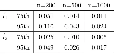
Figure (3.1a) shows the simulation data with the corresponding 25th, 50th and 75th quantile in the red and green dashes from low to high. Figure (3.1b) is the scatter plot of y vs x2. Because bothx2 and y are highly correlated with x1, it is not surprising to see

an obvious correlation betweenx2 and y. Figure (3.1c) and figure (3.1d) are respectively

the estimated 75th quantile functions of the first and second component in 30 simulation replicates. Because local linear regression is subject to boundary effects, the component estimates are very volatile at the both ends. Figure (3.1e) and figure (3.1f) are the average estimated component functions vs. the true functions (dashed lines). The estimates are very close to the true functions on the graphs. To measure the difference between ˆli and

li, integrated squared error,

Z

(ˆli(xi)−li(xi))2dF(xi), i= 1,2

is estimated and summarized in the following Table (3.1), where the estimated ISE goes to 0 as the sample size grows larger.

2. Independence of estimation order: Repeat the same simulation setting as above, but fit x2 as the first component and x1 as the second component. The results show that the

estimations are the same as that of study 1. Although back-fitting algorithm takes an iterative procedure and fits the nuisance variablex2 first, the final solution still converges

(27)

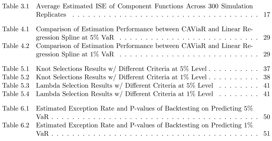
Table 3.1: Average Estimated ISE of Component Functions Across 300 Simulation Replicates

n=200 n=500 n=1000 ˆ

l1 75th 0.051 0.014 0.011

95th 0.110 0.043 0.024 ˆ

l2 75th 0.025 0.010 0.005

95th 0.049 0.026 0.017

3.3.3 Problem with Convergence

Throughout the implementation, the estimation is not always convergent with the backfitting algorithm. In terms of computation, it means convergence criteria are not met (i.e. the differ-ences of the estimations from the last two steps cannot go down below any given threshold). To consider the whole process of the backfitting algorithm, one can note that the procedure does not have a global optimization target, but aims to optimize a different target function (3.3) in each step, in the hope that optimizing in each step will lead to optimizing the global target function (3.1). Therefore, the convergence is not guaranteed. In the simulation settings above, the estimations do not always converge. Even though the halfing step procedure was implemented, the convergence issue is still not solved.

(28)

(a) Data and Quantiles (b) Nuisance variable x2 vs. y

(c) Component functions of x1 (d) Component functions of x2

(e) Averaged component function of x1 (f) Averaged component function of x2

(29)

Chapter 4

Recursive Quantile Regression

Model

4.1 Model Motivation

Recursive models are very popular in time series because they can incoporate long-term de-pendence with a moderate number of parameters, for example, the GARCH model. Nowadays, much literature is devoted to studying models derived from GARCH. Among them, Taylor [1986] and Schwert [1990] proposed TS-GARCH model, which mitigates the influence of large values on the standard deviation by modeling with absolute lagged values instead of quadratic values:

σt=α0+

X

j

αj|rt−j|+

X

i

θiσt−i,

where the underlying assumption is that the data distributions are in the same family that can be fully described by mean and standard deviation. To avoid the distribution assumption, one can substitute σt with the τth-quantile qτ(t). (Denoted as qt as a simplified notation in the

following parts.)

qt=β0+

X

j

βj|rt−j|+

X

i

θiqt−i.

This model above is actually equivalent to model (1.5) where lj(·) is a linear regression

spline with a single knot at 0. Therefore, the model discussed in this work is a more gener-alized form of TS-GARCH, allowing lj to be a regression spline with more than one knot, or

(30)

In this chapter, the estimation procedure of a recursive nonparametric quantile regression will be discussed in detail. As the spline smoothing has the advantage of computing efficiency and alternative linear expressions, we are able to transform the original problem into a solvable linear programming problem. Recursive model with regression spline and smoothing spline will be separately described in the following.

4.2 Recursive model

4.2.1 Estimation with Regression Spline

First consider the simplest case. Suppose the quantile is an additive function of one lagged quantile value and a function of one lagged observation value, that is, whenu= 1 andv= 1 in model (1.5):

qt=θqt−1+l(rt−1),

wheret= 2, ..., T, and parameterβ0 is included in functionl(·).

If the nonparametric component l(·) can be approximated by a regression spline with K basis functions,

l(x) =

K

X

j=1

βjBj(x).

Then, substitute qt−1 with the basis functions recursively, the equation becomes

qt = l(rt−1) +θqt−1

=

K

X

j=1

βjBj(rt−1) +θqt−1

=

K

X

j=1

βjBj(rt−1) +θ





K

X

j=1

βjBj(rt−2) +θqt−2





=

K

X

j=1

βj(Bj(rt−1) +θBj(rt−2)) +θ2qt−2,

and after repeating the substitution (t−2) times,

qt= K

X

j=1

βj t−1

X

i=1

θi−1Bj(rt−i)

!

+θt−1q1. (4.1)

(31)

qt asQt(β, θ), the estimation minimizes T

X

t=1

ρτ(yt−Qt(β, θ)). (4.2)

The estimation of the recursive model is two-staged:

1. Given a grid of θs within (−1,1). that minimizes (4.2), for each θ, estimate the corre-sponding parameter β.

2. The final estimation is the (β,ˆˆθ) that minimizes (4.2).

Usually a two-stage optimization is in concern of reaching at whether the global or local minimization. However, this estimation process does not suffer from this issue. The second stage is minimizing a univariate function ofθwithin a constraint range. If the first stage always derives a global minimum at each given θ, the global minimum of (4.2) can be achieved by a grid search over θ. Note that the first stage is just a classical linear quantile regression, which means that the estimation is a global minimizer of (4.2) at eachθ, so this two-stage estimation will achieve the global minimum with a gird search overθ. As shown in the later Chapter, in real data applications, the second stage univariate function is usually unimodal, so in terms of computational implementation, theR functionoptimize is used instead of brutal grid search algorithm to improve computing efficiency. Estimation with regression spline does not require too much computing effort because it is just a combination of linear quantile regression with transformed design matrix and a minimization of a univariate function.

4.2.2 Estimation with Smoothing Spline

The estimation with smoothing spline, compared to regression spline, is a little more compli-cated and requires much more computing capacity in a single run. Denote the stochastic process {qt}as Q(x|Ft−1), Ft−1={qt−1, qt−2, ..., rt−1, rt−2, ...}, then

Q(x|Ft−1) =l(x) +θQ(rt−1|Ft−2).

Therefore,

dQ(x|F_t−1)

dx =

dl(x) dx

is constant∀t. That is, the smoothness ofQ(x|Ft−1) only depends on l(x) over time. Now the

smoothing spline problem becomes to minimize

T

X

t=1

(32)

Proposition 4.2.1 The minimizer of problem (4.3) is a linear spline with knots at the observa-tions{xi}ni=1 for each fixed θ where g is a function with absolutely continuous first derivatives. Proof IfQ(rt|Ft−1) =qt∗ is fixed, then l(rt) =Q(rt|Ft−1)−θQ(rt−1|Ft−2) =qt∗−θqt∗−1 is also

fixed. Therefore, we can first obtain the form of ˆlthat minimizes the roughness penaltyλV(l0), then what remains is just an interpolation problem to minimize the sum of two parts.

By the same arguments in Koenker et al. [1994], it is straightforward to show the curve that minimizesV(l0) is a piecewise linear interpolator with knots at the observationsrt, and thus it

can also minimize (4.3).

Define an index function it= Argmin l

{r_l :rl> rt}, (t= 1, ..., T −1), i.e. rit is the smallest

value greater thanrt. Without loss of generality, assume that

l(x) =at+bt(x−rt), x∈[rt, rit)

Then,

q2=Q(r1|F1) =l(r1) +θq1=a1+θq1

l0(x)|_x₌_r

1 =b1

q3=Q(r2|F2) =l(r2) +θQ(r1|F1) =l(r2) +θ(a1+θq1) =a2+θa1+θ2q1

l0(x)|_x₌_r

2 =b2

.. .

To summarize,

qt=Q(rt−1|Ft−1) =

t−1

X

i=1

θt−1−iai+θt−1q1, (4.4)

l0(x)|_x₌_r

t−1 =bt−1, (4.5)

where bt=

ait −at

xit −xt

,and t= 2, ..., T. (4.6)

Note the difference of the definition of at and bt in equation (4.6) and in equation (2.4) The

(33)

Define a set of index

{st, t= 1, ..., T−1},s.t. rs1 ≤rs2 ≤...≤rsT−1,

which meanss1 is the time when the return value is the smallest, and s2 is the time when the

return is second smallest, and so on, sT−1 is the time when the return is the largest. Assume

rt values are distinct, then for each rst,

∃m, s.t. rm=rst, and rim =rst+1

Therefore, the model can be estimated following the similar procedures as usual quantile smoothing splines, except that the paramters need to be re-arranged as

a0 = (q1, as1, as2, ...asT−1),

then the total variation part can be written similarly as the second part of equation (2.7) as

λ

T−2

X

j=1

|d0_ja|,

where dj is the same as (2.8) and ht =rst+1−rst, (t= 1, ..., T −1). The estimations can be

obtained by using rqssfuncion inquantreg package of R but need some modification in the functionsrqssandqssto adjust for the changes in the underlying design matrix. The modified function codes are attached in the appendix.

One issue raised in this method is that it requires intensive computing capacity due to the change of design matrix structure. In the original smoothing spline problem, with N observations, the dimension of the design matrix is (2N−2)×N, but in most cells the value is just zero and the R package quantreg is able to use a sparse matrix storage method in order to reduce the memory usage for computation. However, in the recursive model, the quantile function is no longer equal to a singleat value but a summation of all previous values

Pt−1

i1 θ

t−1−i_a

i +θt−1q1. When |θ| is close to 1, the decaying rate of θt−1−i is relatively slow

whenigrows, thus, the design matrix is no longer sparse and the memory requirement is almost

1

2N2 instead of N. Therefore, the algorithm can go over the memory limit very quickly when

the number of observations grows. In approximation, 1000 observation requires around 30G in memory capacity. In order to alleviate this problem, one method is to reparameterize{at}into

{qt}, so that the θt−1−i terms become zeros in the design matrix. This modification saves the

(34)

The modified function of rqssand related codes are attached in the appendix.

4.2.3 Extension to Higher Order

The case whenu >1 orv >1 is not discussed in detail in this work, but the estimation can be extended from the simple caseu= 1 and v= 1.

• When u= 1 andv >1,

qt=θqt−1+

v

X

d=1

ld(rt−d),

the extension is straightforward.

1. Regression Spline: Each link component ld can be estimated by a regression spline

withKd basis functions, then similar to equation 4.1,

qt= v

X

d=1

Kd

X

j=1

βj,d t−1

X

i=1

θi−1Bj,d(rt+1−i−d)

!

+θt−1q1,

and for each fixedθ, estimation can be derived by a linear quantile regression. 2. Smoothing Spline: Each link component ld is a piecewise linear function, then the

estimation is equivalent to additive quantile smoothing spline for each fixedθ. • When u >1 andv= 1,

qt= u

X

s=1

θsqt−s+l(rt−1),

the estimation form remains the same as the case u = 1 and v = 1. As an example, following is a brief description of the estimation whenu= 2 and v= 2.

1. Regression Spline

In analogue to equation 4.1, suppose that the estimation has a general form

qt= K

X

j=1

βjXt,j +W1,tq1+W2,tq2. (4.7)

To substitute this equation in the model

qt=θ1qt−1+θ2qt−2+

K

X

j=1

(35)

so that

qt=θ1(

K

X

j=1

βjXt−1,j+W1,t−1q1+W2,t−1q2)

+θ2(

K

X

j=1

βjXt−2,j+W1,t−2q1+W2,t−2q2) +

K

X

j=1

βjBj(rt−1).

By equating the coefficients ofq1,q2 and {βj}j=1,...,K to the general equation form,

Xt,j =θ1Xt−1,j+θ2Xt−2,j+Bj(rt−1),

W1,t=θ1W1,t−1+θ2W1,t−2,

W2,t=θ1W2,t−1+θ2W2,t−2 fort >2,

and

X1,j = 0, X2,j= 0,

W1,1 = 1, W1,2= 0,

W2,1 = 0, W2,2= 1.

Because the estimation with regression spline is in the form (4.7), it can also be estimated by linear quantile regression given fixed (θ1, θ2), where the design matrices

need more calculations than in the simple case. Now the dimension of the search space in the second stage of the estimation is increased.

2. Smoothing Spline

In analogue to equation 4.6, suppose that the estimation has a general form

qt= t−1

X

j=2

Xt,jaj+W1,tq1+W2,tq2. (4.8)

To substitute this equation in the model

qt=θ1qt−1+θ2qt−2+at−1

(36)

qt=θ1(

t−2

X

j=2

Xt−1, jaj+W1,t−1q1+W2,t−1q2)

+θ2(

t−3

X

j=2

Xt−2, jaj+W1,t−2q1+W2,t−2q2) +at−1.

By equating the coefficients ofq1,q2 and{aj}t=2,...,t−1to the general form, for t >2,

W1,t=θ1W1,t−1+θ2W1,t−2,

W2,t=θ1W2,t−1+θ2W2,t−2

and

Xt,t−1 = 1

Xt,t−2 =θ1Xt−1,t−2 =θ1

Xt,i =θ1Xt−1,i+θ2Xt−2,i for 3≤i≤t−3,

and the initial values are

W1,1 = 1, W1,2= 0,

W2,1 = 0, W2,2= 1.

Again, the estimation is in the form 4.8, that is, the link function can be estimated by linear smoothing spline at given (θ1, theta2), but the design matrix needs more

computations than the simple case.

In summary, the estimations of the recursive model at higher order actually have similar form to that in the simplest case, so the computational procedure described in the previous sections can also be applied to higher order cases. In addition, the model withu= 1 andv = 1 is often found to be sufficient in practice, so this work will mainly focus on the simple case.

4.3 Simulation Study

(37)

methods in a Monte Carlo simulation study. We consider a quantile function

qt= 0.9qt−1+l(rt−1),

wherel(x) = [0.09−0.02xI(x <0) + 0.01xI(x >= 0)]Q(τ),andis from a skewed-t

distribu-tion (µ= 0, σ= 2, ν = 6.35, ξ =.92). (Q(0.05) =−3.29, Q(0.01) =−5.38) So to rewrite it in

the form of

qt=β1+β2qt−1+β3(rt−1)++β4(rt−1)−,

forτ =.05,

β1 =−0.30, β2 = 0.9, β3 =−0.033, β4 =−0.066,

forτ =.01,

β1 =−0.48, β2 = 0.9, β3=−0.054, β4 =−0.108

The observations{rt} can be generated recursively as follows

r1 =1,

q1 =Q(τ),

fort≥2, andk= 1,2

rt={[0.9qt−1+l(rt−1)]/Q(τ)}t

qt= 0.9kt−1+l(rt−1),

where{_t} are independently generated from the skewed-t distribution.

In order to study how the estimation performance is influence by the sample size, data are generated with three different size (n= 250,500,1000), and for each size we have 300 replicates. Quantiles are estimated at both 1% and 5% level by two methods, CAViaR with Asymmetric Slope and Linear Spline Regression with knot fixed at 0. The goodness of fit is measured by the Average Absolute Deviation (AAD) of estimation from the true quantile values,

AAD(ˆq{method}) =

T

X

t=1

|ˆqt{method} −qt{method}|/T, (4.9)

whereT = 1000 in this simulation.

(38)

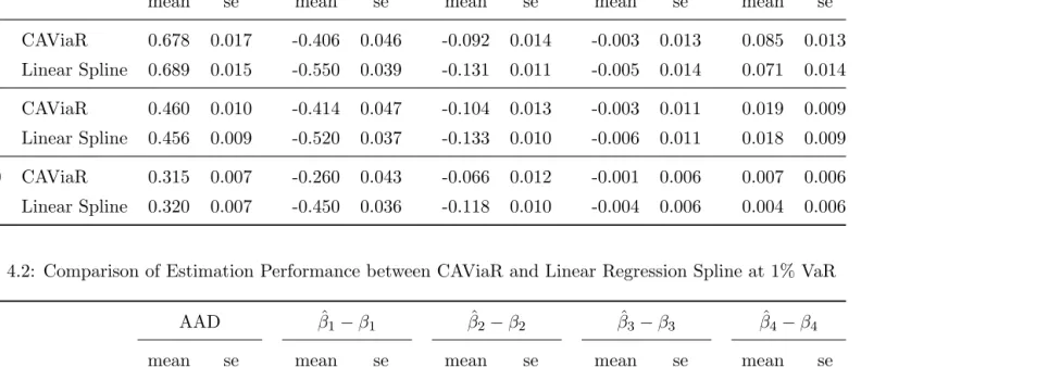
n= 250, and the improvement is milder from n= 500 to n= 1000. When in the case n= 500 and n = 1000, the estimation of β3 and β4 is reasonably approximating to the true value.

However, there is no implication that the estimation of β1 and β2 can be improved when n

(39)

Table 4.1: Comparison of Estimation Performance between CAViaR and Linear Regression Spline at 5% VaR

AAD βˆ1−β1 βˆ2−β2 βˆ3−β3 βˆ4−β4

mean se mean se mean se mean se mean se

n=250 CAViaR 0.678 0.017 -0.406 0.046 -0.092 0.014 -0.003 0.013 0.085 0.013

Linear Spline 0.689 0.015 -0.550 0.039 -0.131 0.011 -0.005 0.014 0.071 0.014

n=500 CAViaR 0.460 0.010 -0.414 0.047 -0.104 0.013 -0.003 0.011 0.019 0.009

Linear Spline 0.456 0.009 -0.520 0.037 -0.133 0.010 -0.006 0.011 0.018 0.009

n=1000 CAViaR 0.315 0.007 -0.260 0.043 -0.066 0.012 -0.001 0.006 0.007 0.006

Linear Spline 0.320 0.007 -0.450 0.036 -0.118 0.010 -0.004 0.006 0.004 0.006

Table 4.2: Comparison of Estimation Performance between CAViaR and Linear Regression Spline at 1% VaR

AAD βˆ1−β1 βˆ2−β2 βˆ3−β3 βˆ4−β4

mean se mean se mean se mean se mean se

n=250 CAViaR 1.418 0.037 -0.413 0.068 -0.061 0.012 -0.006 0.027 0.085 0.029

Linear Spline 1.443 0.036 -0.807 0.065 -0.126 0.011 -0.015 0.031 0.073 0.031

n=500 CAViaR 0.996 0.024 -0.532 0.067 -0.090 0.012 -0.042 0.024 0.006 0.020

Linear Spline 1.021 0.022 -0.943 0.066 -0.154 0.010 -0.028 0.024 0.018 0.023

n=1000 CAViaR 0.735 0.018 -0.437 0.066 -0.071 0.011 -0.016 0.016 0.010 0.013

(40)

Chapter 5

Selection of Smoothing Parameter

5.1 Introduction

Although a nonparametric estimation method can be free from assumptions on the data distri-bution or functional form, the goodness of the fit is still affected by the smoothing parameter, or tuning parameter. In regression spline, the smoothing parameters are the number of knots K and their locations, which determine the structural change in the shape of the fitted curve; with smoothing parameter, the smoothing parameter isλ, which controls the smoothness of the fitted curve, or the dimension of the effective model. While in local linear models with kernel weighting, the smoothing parameter ish, the window width that implicitly controls the number of observations to be included in the local linear fitting. In a word, the smoothing parameters determine the model dimension in nonparametric regressions.

Selection of smoothing parameters is a very critical step in nonparametric regressions. Al-though it can be sometimes selected subjectively according to the past studies or experiences, an automatic procedure of selecting smoothing parameters driven by data is still highly de-sirable. Then the question is what makes a good choice of the smoothing parameter. One could possibly allow the nonparametric regression model large enough so that the estimates will interpolate every observation: when K = N −2, λ = 0 or h is small enough. Although this type of model has very good fit in the training data, they are too specified for the sample data and usually have poor performance in the prediction. After all, the purpose of fitting a nonparametric model is to discover the associations in the current data, and make further prediction or inference when new observations come in, so a good nonparametric model should have good prediction power. While this power can be evaluated by the expected prediction error:

Eρτ(y−g(x)),ˆ

(41)

this value is not achievable because the true underlying distribution is unknown, but it can be approximated by Monte Carlo method as sampling an additional test data set (really large enough data set) which are distributed identically and independent from the training data. Then the GC of ˆg can be estimated by

Ntest

X

i=1

ρτ ytest−ˆg(xtest)

/Ntest. (5.1)

Though this value is usually not attainable, it can be used here as a reference to compare between different smoothing parameters selection methods. Another way to approximate the expected prediction error is cross-validation(CV), because it is a measure of the average predic-tion power when one observapredic-tion is crossed out from the training data. However, this procedure is very time-consuming. In order to attenuate this issue, many criteria have been proposed to approximate CV, say AIC, BIC, ACV and GCV.

Since nonparametric method has attracted more and more interest in real application, many studies have been devoted into discussing the automatic selection of smoothing parameters. Compared to the mean regression settings, there is rather limited literature about smoothing parameter selection in quantile regression settings. Koenker et al. [1994] first suggested the SIC (Scharwz Information Criterion) to be used to select optimal λ in quantile smoothing spline and was commonly used by many following studies. He and Shi [1994] also suggested using SIC in regression B-spline estimation.

SIC = log( 1 N

X

i

ρτ(yi−ˆg(xi))) +

1

2Rlog(N)/N, (5.2)

whereRis the model dimension . Cai and Xu [2009] later proposed to select a bandwidth for the kernel smoothing estimation with an improved AIC (Akaike Information Criterion) (Hurvich et al. [1998]):

AIC = log( 1 N

X

i

ρτ(yi−ˆg(xi))) +

2(R+ 1)

N−(R+ 2). (5.3)

(42)

observations goes to infinity from a limited number of candidate pool in M-estimators. Although there is a gap between the SIC criterion in this paper and the one used by Koenker et al. [1994], the goodness-of-fit part of the latter one is actually an analogue of the likelihood when the data distribution is double exponential. In addition, because of the ease of computation and previous success in numerous empirical analysis, SIC is still the most commonly used in model selection of quantile models. A recent development, Yuan [2006], introduced the estimation of GACV (Generalized Approximate Cross-Validation) for smoothing quantile. In that work, they have compared the GACV with AIC and SIC in real data application and found that GACV and SIC have very similar results in the model selection. The only problem with the GACV is the intuitive explanation of this value when the data is time series type. Therefore, we suggest using SIC, by Koenker et al. [1994] and He and Shi [1994] as the criterion to select the optimal smoothing parameters.

5.2 Knot Selection in Regression Spline

5.2.1 Introduction

In past studies, the number of knots and knot locations have been recognized to greatly influence the estimation and prediction of regression splines, because misspecified knots is equivalent to misspecified curve structures and will lead to a biased estimation. Because deleting or adding one knot leads to a different model (especially in B-spline regression, the Basis functions are all influenced by the addition or deletion one knot), givenK knots, the knot selection procedure is equivalent to model selection from 2K candidate models, which is a very challenging problem even whenKis a moderate value. Among many possible procedures that help avoid to directly select from a pool of 2K candidate models, there are two most popular methods for knot selection:

1. Stepwise Selection

First specify a maximum numberM(usuallyM = 9), then choose the optimal model from a pool of candidate models with{0,1,2,...,M}number of internal knots that are uniformly distributed in percentage or Euclidean distance. For example, a model with 9 internal knots uniformly distributed in percentage has the knots located at the 10%, 20%, ..., 90% quantiles. Then starting from this selected model, cycle the knot deletion and addition steps until the target value cannot be improved any further. If the target value is SIC, then the procedure will cycle until SIC cannot be reduced any further.

(43)

the procedure until SIC does not decrease if removing any knot.

(b) Step 2: Stepwise knot addition. Consider the midpoint of two adjacent knots (in terms of percentile of Euclidean distance) as potential knots and add the one that improves the target value best. Repeat the procedure until no more knots can be added.

2. Penalized Shrinkage

Given truncated polynomial basis, the estimated function is

ˆ g(x) =

p

X

i=0

αixi+ K

X

k=1

αpk(x−ξk)p+,

A small absolute value of αpk corresponds to a small impact of kth knot in pthe order.

Penalizing on the parameters αpk is equivalent to penalizing on the smoothness of the

fitted function, therefore, an idea to develop an optimal criterion is as follows,

ρτ(yi−gˆλ(xi)) +γ K

X

k=1

α2_pk, (5.4)

thenγ controls the extent of smoothness. The selection of knots location is now reduced to the selection ofγ. Because this procedure is not instantly applied to B-spline basis, in the following discussion, we will continue to discuss using the Stepwise Selection for knot selection.

5.2.2 Selection in Recursive Model

As discussed in Chapter (4), the recursive model with the link function as a regression spline can be re-written as a modified regression spline. Therefore, the smoothing parameter selection methods in traditional regression spline can also be applied to the model selection of recursive model.

In terms of model dimension, the recursive model indeed increases the number of parameters. Specifically, the recursive model has additional lagged quantile variables to the non-recursive one, and therefore requires more parameters estimations. In calculating the effective model di-mension,R, we need to count in all estimated parameters. Except for the estimated parameters from regression spline, θ and q1 are also estimated in the model as parameters. For example,

(44)

In fact, SIC can also be used to identify the significant lagged variables in the model, because the selection of number of lagged variables is also a procedure of model selection.

5.2.3 Simulation Study

Current studies on smoothing parameter selections for nonparametric quantile regression mainly focus on quantile levels such as the median and quartiles, and the behavior of the criteria were examined given the predictor variables are uniformly or normally distributed. However, in our setting, the predictor and responses are time series data and our interest is to apply it to financial data. In fact, the distribution of financial data are usually asymmetric and fat-tailed, as shown in the scatter plot of (6.3). Obviously, we are facing the challenge that data at both ends of the range is very sparse and a lot of data points are clustered close to the median. Therefore, in this section, a simulation study will be carried out to evaluate the current smoothing parameter selection criteria under a setting close to the real-world data, say S&P 500.

The simulation data are generated as follows:

• We consider the quantile processes as

q_tk= 0.9qk_t−1+lk(rt−1),

and l1 and l2 are two different link functions:

l1(x) = [0.09−0.02xI(x <0) + 0.01xI(x >= 0)]Q(τ),

l2(x) =

h

0.28−0.18 cos(π 10x)

i Q(τ),

so we have two different processes in this simulation study.

Accordingly, the observations {r_t}can be generated recursively as follows

r1 =1,

q₁k=Q(τ),

fort≥2, andk= 1,2

rt={[0.9qt−1+lk(rt−1)]/Q(τ)}t

qk_t = 0.9q_tk₋₁+lk(rt−1),

where {t}, are independently generated from a skewed-t distribution (µ= 0, σ= 2, ν =

(45)

In the graph (5.1) gives the scatterplot of a sample data and the function curves of 1%(green dotted) and 5%(red dashed) quantiles. Notice that l1(x) is a piecewise linear

function with the structure change point at 0 and the function is not symmetric about 0, and l2(x) has more curvature than l1(x) and is symmetric about 0. Therefore, our

simulation result will cover both linear and nonlinear type of nonparametric functions and the comparisons will not be in favor of a particular model that is in nature closer to the underlying function. For example, the linear spline model may work better on estimatingq1 than natrual cubic spline.

• For each process, generate 300 data sets with 1500 observations in each. The first 1000 observations are then used for training, called training data, while the remaining 500 observations are test data.

• With each training data, quantiles are estimated at both 1% and 5% level . Each fit is

called a replicate, so this simulation has 300 replicates for each process. The test data is then used for choosing the best smoothing parameters by the Gold Criterion.

• For each replicate, use the Gold Criterion (GC), SIC and AIC separately to choose the number of knots and knot locations, and fit 3 different models corresponding to the selected knots by different criteria.

• The goodness of fit is measured by the Average Absolute Deviation (AAD) of estimation

from the true quantile values,

AAD(ˆqk{knots}) =

T

X

t=1

|ˆq_tk{knots} −qk_t{knots}|/T, (5.5)

wherek= 1,2 andT = 1000 in this simulation.

(46)

● ● ● ● ● ● ● ● ● ● ● ● ● ● ● ● ● ● ● ● ● ● ● ● ● ● ● ● ● ● ● ● ● ● ● ● ● ● ● ● ● ● ● ● ● ● ● ● ● ● ● ● _● ● ● ● ● ● ● ● ● ● ● ● ● ● ● ● ● ● ● ● ● ● ● ● ● ● ● ● ● ● ● ● ● ● ● ● ● ● ● ●●● ● ● ● ● ● ● ● ● ● ● ● ●●● ● ● ● ● ● ● ● ● ● ● ●● ● ● ● ● ● ● ● ● ● ● ● ● ● ● ● ● ● ● ● ● ●● ● ● ● ● ● ● ● ● ● ● ● ● ● ● ●● ● ● ● ● ● ● ● ● ● ● ● ● ● ● ● ● ● ● ● ● ● ● ● ● ● ● ● ● ● ● ● ● ● ● ● ● ● ● ● ● ● ● ● ● ● ● ● ● ● ● ● ● _● ● ● ● ● ● ● ● ● ● ● ● ● ● ● ● ● ● ● ● ● ● ● ● ● ● ● ● ● ● ● ● ● ● ● ● ● ● ● ● ● ● ● ● ● ● ● ● ● ● ● ● ● ● ● ● ● ● ● ● ● ● ● ● ● ● ● ● ● ● ● ● ● ● ● ● ● ● ● ● ● ● ● ● ● ● ● ● ● ● ● ● ● ● ● ● ● ● ● ● ● ● ● ● ● ● ● ● ● ● ● ● ● ● ● ● ● ● ● ● ● ● ● ● ● ● ● ● ●●● ● ● ● ● ● ● ● ● ● ● ● ● ● ● ● ● ● ● ● ● ● ● ● ● ● ● ● ● ● ●● ● ● ● ● ● ● ● ● ● ● ● ● ● ● ● ● ● ● ● ● ● ●● ● ● ● ● ● ● ● ● ● ● ● ● ● ● ● ● ● ●● ● ● ● ● ● ● ● ● ● ● ● ● ● ● ● ● ● ● ● ● ● ● ● _● ● ● ● ● ● ● ● ● ● ● ● ● ● ● ● ● ● ● ● ● ● ● ● ● ● ● ● ● ● ● ● ● ● ● ● ● ● ● ● ● ● ● ● ● ● ● ● ● ● ● ● ● ● ● ● ● ● ● ● ● ● ● ● ● ● ● ● ● ● ● ● ● ● ● ● ● ● ● ● ● ● ● ● ● ● ● ● ● ● ● ● ● ● ● ● ● ● ● ● ●● ● ● ● ● ●● ● ● ● ● ● ● ● ● ● ● ● ● ● ● ● ● ● ● ● ● ● ● ● ● ● ● ● ● ● ● ● ● ● ● ● ● ● ● ● ● ● ● _●●● ● ● ● _● ● ● ● ● ● ● ● ● ● ● ● ● ● ● ● ● ● ● ● ● ● ● ● ● ● ● ● ● ● ● ● ● ● ● ● ● ● ● ● ● ● ● ● ● ●● ● ● ● ● ● ● ● ● ● ● ● ● ● ● ● ● ● ● _● ● ● ● ● ● ● ● ● ● ● ● ● ● ● ● ● ● ● ● ● ● ● ● ● ● ● ● ● ● ● ● ● ● ● ● ● ● ● ● ● ● ● ● ● ● ● ● ● ●● ● ● ● ● ● ● ● ● ● ● ● ● ● ● ● ● ● ● ● ● ● ● ● ● ● ● ● ● ● ● ● ● ● ● ● ● ● ● ● ● ● ● ● ● ● ● ● ● ● ● ● ● ● ● ● ● ● ●● ● ● ● ● ● ● ● ● ● ●_● ● ● ● ● ● ● ● ● ● ● ● ● ● ● ● ● ● ● ● ● ●● ● ● ● ● ● ● ● ●● ● ● ● ● ● ● ● ● ● ● ● ● ● ● ● ● ● ● ● ● ● ● ● ● ● ● ● ● ● ● ● ● ● ● ● ● ● ● ● ● ● ● ● ● ● ● ● ●●● ● ● ● ● ● ● ● ● ● ● ● ● ● ● ● ● ● ● ● ● ● ● ● ● ● ● ● ● ● ● ● ● ● ● ● ● ● ● ● ● ● ● ● ● ● ● ● ● ● ● ● ● ● ● ● ● ● ● ● ● ● ● ● ● ● ● ● ● ● ● ● ● ● ● ● ● ● ● ● ● ● ● ● ● ● ● ● ● ● ● ● ● ● ● ● ● ● ● ● ● ● ● ● ● ● ● ● ● ● ● ● ● ● ● ● ● ● ● ● ● ● ● ● ● ● ● ● ● ● ● ● ● ● ● ● ● ● ● ● ●

−10 −5 0 5 10

−10

−5

0

5

10

Process by l1

rt−1 rt ● ● ● ● ● ● ● ● ● ● ● ● ● ● ● ● ● ● ● ● ● ● ● ● ● ● ● ● ● ● ● ● ● ● ● ● ● ● ● ● ● ● ● ● ● ● ● ● ● ● ● ● ● ● ● ● ● ● ● ● ● ● ● ● ● ● ● ● ● ● ● ● ● ● ● ● ● ● ● ● ● ● ● ● ● ● ● ● ● ● ● ●●● ● ● ● ● ● ● ● ● ● ● ● ●●● ● ● ● ● ● ● ● ● ● ● ●● ● ● ● ● ● ● ● ● ● ● ● ● ● ● ● ●● ● ● ● ●● ● ● ●_● ● ● ● ● ● ● ● ● ● ● ●● ● ● ● ● ● ● ● ● ● ● ● ● ● ● ● ● ● ● ● ● ● ● ● ● ● ● ● ● ● ● ● ● ● ● ● ● ● ● ● ● ● ● ● ● ● ● ● ● ● ● ● ● ● ● ● ● ● ● ● ● ● ● ● ● ● ● ● ● ● ● ● ● ● ● ● ● ● ● ● ● ● ● ● ● ● ● ● ● ● ● ● ● ● ● ● ● ● ● ● ● ● ● ● ● ● ● ● ● ● ● ● ● ● ● ● ● ● ● ● ● ● ● ● ● ● ● ● ● ● ● ● ● ● ● ● ● ● ● ● ● ● ● ● ● ● ● ● ● ● ● ● ● ● ● ● ● ● ● ● ● ● ● ● ● ● ● ● ● ● ● ● ● ● ● ● ● ● ●● ●●●●● ● ● ● ● ● ● ● ● ● ● ● ● ● ● ● ● ● ● ● ● ● ● ● ● ● ● ● ● ●● ● ● ● ● ● ● ● ● ● ● ● ● ● ● ● ● ● ● ● ● ●● ● ● ● ● ● ● ● ● ● ● ● ● ● ● ● ● ● ● ●● ● ● ● ● ● ● ● ● ● ● ● ● ● ● ● ● ● ● ● ● ● ● ● ● ● ● ● ● ● ● ● ● ● ● ● ● ● ● ● ● ● ● ● ● ● ● ● ● ● ● ● ● ● ● ● ● ● ● ● ● ● ● ● ● ● ● ● ● ● ● ● ● ● ● ● ● ● ● ● ● ● ● ● ● ● ● ● ● ● ● ● ● ● ● ● ● ● ● ● ● ● ● ● ● ● ● ● ● ● ● ● ● ● ● ● ● ● ● ● ● ● ● ● ●● ● ● ● ● ●● ● ● ● ● ● ● ● ● ● ● ● ● ● ● ● ● ● ● ● ● ● ● ● ● ● ● ● ● ● ● ● ● ● ● ● ● ● ● ● ● ● ● _●●● ● ● ● _● ● ● ● ● ● ● ● ● ● ● ● ● ● ● ● ● ● ● ● ● ● ● ● ● ● ● ● ● ● ● ● ● ● ● ● ● ● ● ● ● ● ● ● ● ●● ● ● ● ● ● ● ● ● ● ● ● ● ● ● ● ● ● ● ● ● ● ● ● ● ● ● ● ● ● ● ● ● ● ● ● ● ● ● ● ● ● ● ● ● ● ● ● ● ● ● ● ● ● ● ● ● ● ● ● ● ● ● ● ● ● ● ● ● ● ● ● ● ● ● ● ● ● ● ● ● ● ● ● ● ● ● ● ● ● ● ● ● ● ● ● ● ● ● ● ● ● ● ● ● ● ● ● ● ● ● ● ● ● ● ● ● ● ● ● ● ● ● ● ● ● ● ●● ● ● ● ● ● ● ● ● ● ● ● ● ● ● ● ● ● ● ● ● ● ● ● ● ● ● ● ● ● ● ● ●● ● ● ● ● ● ● ● ● ● ● ● ● ● ● ● ● ● ● ● ● ● ● ● ● ● ● ● ● ● ● ● ● ●_● ● ● ● ● ● ● ● ● ● ● ● ● ● ● ● ● ● ● ● ● ● ● ●●_●● ● ● ● ● ● ● ● ● ● ● ● ● ● ● ● ● ● ● ● ● ● ● ● ● ● ● ● ● ● ● ● ● ● ● ● ● ● ● ● ● ● ● ● ● ● ● ● ● ● ● ● ● ● ● ● ● ● ● ● ● ● ● ● ● ● ● ● ● ● ● ● ● ● ● ● ● ● ● ● ● ● ● ● ● ● ● ● ● ● ● ● ● ● ● ● ● ● ● ● ● ● ● ● ● ● ● ● ● ● ● ● ● ● ● ● ● ● ● ● ● ● ● ● ● ● ● ● ● ● ● ● ● ● ● ● ● ● ● ●

−20 −15 −10 −5 0 5 10

Process by l2

rt−1

rt

(a) Scatter Plot of Simulated Data

−10 −5 0 5 10

−1.6 −1.4 −1.2 −1.0 −0.8 −0.6 −0.4 x l1 ( x )

−10 −5 0 5 10

−2.5 −2.0 −1.5 −1.0 −0.5 x l2 ( x )

(b) Link Functions