A programming system for parallel digital signal processor networks

A

Programming System for Parallel

Digital Signal Processor Networks

Todd

A.

Cook

Center for Commuinications and Signal Processing

Department of Electrical and Computer Engineering

North Carolina State University

COOK, TODD A. A Programming System for Parallel Digital Signal Processor Networks (Under the direction of Thomas K. Miller III.)

A system, called PaLS, has been developed for programming parallel digital signal processor networks. This system consists of a psuedo-compiler for a newly designed, C-like language (called DFC), an algorithm partitioner, a scheduler, and a code generator.

Contents

List Of Figures

...

III

List Of Tables iv

1 Introduction 1

2 The PaLS Programming System 4

2.1

Data Representation 4

2.2

Algorithm Input 6

2.3

Partitioning . . . 6

2.4

Link Assignment 9

2.5

Scheduling . . . .

...

9

3 Modifications to PaLS 11

3.1

Data Representation

12

3.2

Algorithm Input

..

.

....

14

3.2.1

Language Requirements

15

3.2.2

Existing Languages .

15

3.2.3

The D

Fe

Language 16

3.2.4

IR Optimizer

...

17

3.2.5

IR Linker

....

18

3.3.1 Mean Field Annealing . . . . . 3.3.2 Mean Field Annealing Performance. 3.4 Scheduling . . . .

3.5 Code Generation

4 Trial Runs 4.1 IIR Filter 4.2 LMS Filter 4.3 Adder Tree

5 Discussion and Further Work 5.1 The DFC Language .

5.1.1 Discussion of DFC · 5.1.2 Further Work on DFC . 5.2 Partitioning...

A DFC Reference Manual

A.I Lexical Conventions

A.I.I Comments.

A.l.2 Identifiers · A.1.3 Reserved Words

A.l.4 Constants

A.2 Variables · A.3 Expressions

A.3.1 Operators

A.3.2 Precedence Rules ·

A.4 Declarations . . A.5 Statenaents A.6 Functions .. A.7 Scope Rules.

A.8 A DFC Grammar ..

B IR Reference Manual

B.l Node Names

...

B.2 The main Section B.3 Function Definitions

B.4 IR Statements.

..

B.4.1 Expressions

..

B.4.2 Function Calls B.4.3 Operators

B.4.4 Input/Output . . B.5 IR Grammar

..

. .

C PaLS Programs

c.i

DCC - Compiler/Linker/Optimizer Control

C.2 DFC - DFC Compiler C.3 OPT - IR Optimizer C.4 LNK - IR Linker

...

C.5 PAS - Partitioner Control C.6 RNO - IR Renumberer . C.7 MFA - Partitioner

...

C.8 SCH - Program Scheduler

...

C.9 IRC - IR to C Converter . . .

D.I Delays . . .

...

63

D.2 Parallel-Cascade IIR Filter 63

E PaLS Standard Library 67

F Glossary 69

List of Figures

2.1 Organization of PaLS 5

2.2 Example Flow-graph . . 5

3.1 Organization of the Modified PaLS System 12

3.2 Run Time vs. Number of Nodes for MFA 25

4.1 Parallel-Cascade IIR Filter 28

4.2 4-Tap LMS Filter . . 29

4.3 63 Node Adder Tree 30

D.I 3x3 Parallel-Cascade IIR Filter 64

D.2 Biquad Filter Section. . . 64

3.1 Number of Bad Annealing Runs 22 3.2 MFA vs. Simulated Annealing: Average Execution Time (Seconds). 23 3.3 MFA vs. Simulated Annealing: Average Number of External Edges. 23 3.4 MFA vs. Simulated Annealing: Average Bin Imbalance 23

4.1 Results of Partitioning the IIR Filter. 4.2 Results of Partitioning the LMS Filter 4.3 Results of Partitioning the Adder Tree .

28

29

30

A.I Operator Precedence · . · . . 42

B.1 IR Operators · · · . . 51

Chapter

1

Introduction

There are two general approaches to achieving high computational speed: using a single high-speed processor (such as a Cray-l or a Cyber 205) or using a large number of relatively low-speed processors operating in parallel (such as the MPP or an NCube). Machines using the former approach tend to be easier to program, but they tend to be expensive to purchase and operate because of the exotic technologies used to make them. Machines using parallel processors are relatively inexpensive because they can be made from off-the-shelf microprocessors; however, they are harder to program because the programmer must design his algorithms to match the communication structure of the machine.

Both the approaches to achieving high speed can be applied to digital signal processing. However, many DSP applications (military, modems, etc.) are for em-bedded systems where cost (in terms of dollars, power consumption, physical space,

etc.) is a major consideration. A parallel approach is therefore desirable because the DSP systems could be built from several low-cost, off-the-shelf processing ele-ments. There are now a number of such processors that are commercially available; for applications using integer arithmetic, some available processors are

• TMS320C25 also from Texas Instruments

• DSP56000 from Motorola

• ADSP-2100 from Analog Devices

• DSP16 from AT&T

while for floating-point applications, some processors are

• TMS320C30 from Texas Instruments

• DSP96000 from Motorola

• DSP32 from AT&T

• p,PD77230 from NEe

The use of such parallel DSP systems, however, is complicated by the need to determine an efficient connection scheme and by the ne-rd to efficiently partition the algorithm to run on the processor network. It would therefore be desirable to have an automatic tool to determine an efficient communication topology and algorithm partitioning.

CHAPTER 1. INTRODUCTION 3

functions to represent computations; a more natural textual method of describing algorithms would be desirable. Partitioning is performed using the simulated

an-nealing process [Kir83]; this process produces near-optimal results, but it is slow and a faster algorithm would improve performance. Finally, PaLS does not produce executable code, so that a way to generate object code is necessary.

This thesis presents a number of improvements made to PaLS. A new language, called DFC, has been developed for expressing signal processing algorithms in a form that is amenable to partitioning. Simulated annealing has been replaced by mean field annealing [Bou88]; this algorithm is one to two orders of magnitude faster than simulated annealing. Many of the DSP vendors are now offering C compilers for their DSPs; therefore, a C code generator has been added that will generate a C program for each of the partitions.

The PaLS Programming System

The PaLS Programming System was developed by David E. Van den Bout as part of his doctoral thesis [Bou87]. The system automatically maps an algorithm onto a network of processing elements and derives the communication topology for the processors. The system then schedules the operations of the algorithm upon the processors with the aim of maximizing throughput and eliminating the potential for deadlock to occur. Figure 2.1 shows the organization of PaLS.

2.1

Data Representation

PaLS represents algorithms as flow-graph3. A flow-graph is a directed graph whose

nodes represent operations (such as addition or subtraction) and whose arcs, or

edqe», represent data flow from one operation to the next. The operations are atomic (indivisible); there is no reason a node could not represent a more complex operation, but no method for doing so is specified. As a small example, the program

fragment

a

:= (b

+

c) •

3;

d := e

-1-

8;

CHAPTER 2. THE PALS PROGRAMMING SYSTEM

Algorithm

Figure 2.1: Organization of PaLS

5

e

b

c

3

Each node and edge has an associated weight. The weight of a node represents its computational cost; that is, it specifies how much time the operation will take to perform. The weight of an edge represents the amount of information (or number of data items) that the edge will carry.

The flow-graphs are stored as a list of nodes (each of which is numbered) and edges. The entry for a node contains its number, weight, and operation; the entry for an edge contains the number of the source node, the number of the- destination node, the edge weight, and the edge direction.

2.2

Algorithm Input

PaLS provides two methods for expressing algorithms: graphically and textually. The graphical method uses a general-purpose graphical editor to enter a signal flow graph describing the algorithm; another program then extracts the flow-graph from the output of the editor. The textual method uses special purpose C functions to describe the algorithm in terms of the nodes; when the C program is compiled and run, it produces a flow-graph representing the algorithm.

2.3

Partitioning

The partitioning phase of PaLS is the process of assigning each node of a flow-graph to a processor for execution. This process consists of finding a balance between two

opposing constraints:

• Processor loads should be equal, or balanced. Balance is desired so that no processor will sit idle wasting cycles while other processors are doing work .

CHAPTER 2. THE PALS PROGRAMMING SYSTEM 7

transfer the data and the hardware needed.

Communications could be trivially minimized by assigning all of the computations to a single processor, in which case there would be no communications costs at all (and no point in a parallel architecture); however, if perfect balance were achieved without regard to communications penalties, then the number of inter-processor communications is iikely to be high. Therefore, the two desired objectives play against each other, and any partitioning will be a tradeoff between them.

The quality of any given partition is described by an objective function, H, that represents the costof the partition. A general form that represents the above problem is [Bou87]

where

He

==

cost of edges between processors Hb

==

cost of processor imbalance

a:

==

scale factor representing the relative significance of processor imbalance

The partitioning process is therefore the process of finding the partition with the smallest cost. However, the search is complicated by the possible existence of local minima in the objective function; the search may become stuck in one of these

local minima even though a better, lower cost solution may exist. This complication makes the process an NP-complete problem; that is, an increase in the number of nodes causes an exponential increase in the search time. Therefore, a means of finding a near-optimal solution is required.

technique for solving combinatorial problems (like graph partitioning) by viewing them as physical systems seeking a low energy state. The annealing of metals or the growing of crystals starts with a molten, disordered collection of particles at a high temperature which, through thermal agitation combined with a slow cooling process, arrives at a highly ordered solid state with low internal energy. This can be likened to the random movement of graph nodes between bins until a good partition with a low value of H is obtained. ([Bou87], page 143)

A high level description of the simulated annealing algorithm is as follows [Bou87]:

1. Create a random partitioning of the flow-graph.

2. Randomly select a node and move it to a randomly chosen bin (processor).

3. Evaluate the cost of the new configuration. If the cost has decreased, accept the move. Otherwise, generate a random number, r, and compare it to e

¥,

where T is the temperature; if r

<

e¥, then accept the move, otherwise,

reject it.

4. Repeat the above step until equilibrium is attained. The system is in

equilib-rium when the average cost is no longer decreasing.

5. Decrease the temperature. If the system is frozen, then stop. The system is frozen when there is no longer any decrease in the average cost as the

temperat ure is decreased.

CHAPTER 2. THE PALS PROGRAMMING SYSTEM 9

of the system in hope of not getting stuck in local minima. More detailed, theoretical treatments can be found in [Kir83] and [Bou87]; [Bou87] (pages 143-152 and 204-212) provides guidelines for applying simulated annealing to the partitioning of flow-graphs.

2.4

Link Assignment

PaLS was designed to work with a custom DSP designed by Dr. Van den Bout. One of the features of this design is that it allows the bandwidth of the inter-processor communications (IPC) port to be allocated to different communication links; that is, the 16-bit port could be divided into a combination of 1, 2, 4, 8, and 16 bit data "links. The link assignment phase of PaLS allocates these variable width data links based upon the partition found in the previous phase; the objective is to assign higher bandwidth links to heavily used or time critical communication paths in order to minimize the delay caused by communication.

However, commercial DSP's do not have variable width IPC ports, and the objective here is to modify PaLS for use with commercial products. Therefore, link assignment is not present in the modified version of PaLS, and it will not be discussed further here. For further details, see pages 153-159 of [Bou87].

2.5

Scheduling

Chapter

3

Modifications to PaLS

A number of modifications have been made to PaLS to improve its usability and its performance. The modifications are

• The format for representing algorithms has been changed. Instead of using explicit flow-graphs, algorithms are now represented by a series of prefix ex-pressions.

• Algorithms are now expressed in a new language called DFC. This language allows a direct textual representation of the algorithm.

• Mean field annealingis now used to do the partitioning. This method derives equally good results an order of magnitude faster.

• The link assignment phase has been removed because commercial DSP's do not have the variable sized IPC ports that PaLS was designed to work with.

• The scheduler was modified to reflect the changes made in algorithm repre-sentation.

• A code generation step has been added. A C program for each processor is now produced.

Algorithm

Figure 3.1: Organization of the Modified PaLS System

3.1

Data Representation

Large programs are a problem to partition because the corresponding flow-graphs are large, and the larger the flow-graph, the longer it takes to partition. One ap-proach to limiting flow-graph size is to allow nodes to represent complex operations; such a node is called a supernode.

Supernodes allow complex expressions to be represented by a single node. For example, without supernodes the statement

a==b+c*(d+1)

CHAPTER 3. MODIFICATIONS TO PALS

d

13

1

c

b

a

whereas if the statement were put into a supernode, it would be represented by

c

d

b

a

1

Therefore, by putting such expressions into a single node, the size of flow-graphs

and the time needed to partition them can be reduced.

description has been changed so that it may now contain an arbitrary expression whose operands are explicitly specified by name; the weight of a node is now the sum of the weights of the operations contained in that node. With this modification, a node may now represent a single operation as before or a complex expression with several operators; in either case, the node will appear as a single, indivisible entity to the partitioner.

The format for storing flow-graphs has been drastically modified to accommo-date supernodes. Since a node description now contains the names of its operands, explicit storage of edges is no longer necessary. Explicit storage of a node's weight is also not required; programs that manipulate flow-graphs can calculate node weights from a global table of operator weights.

The new flow-graph representation is called the intermediate representation, or IR. This form is simply a list of prefix expressions, each of which represents a node. For example, the statement

a==b+c*(d+l)

would be represented in the IR format by

(== a

(+

b

(*

c

(+

d 1))))

(except that the operands are represented by node numbers instead of node names). A complete description of the IR can be found in Appendix B.

3.2

Algorithm Input

CHAPTER 3. MODIFICATIONS TO PALS

15

way of expressing DSP algorithms would be through a conventional programming language.

3.2.1

Language Requirements

There are several requirements that a language must meet to be used with PaLS. These requirements are

1. It must be capable of easily expressing DSP algorithms.

2. It should be compatible with PaLS's view of programs as flow-graphs.

3. It should be machine independent.

4. It should not require programmers to explicitly express parallelism.

5. It should not be strange.

The last two requirements are to ensure that the language is easy to learn and use; explicit expression of parallelism is not required so that programmers will not be forced to learn new programming styles (and because the whole goal of PaLS is to do automatic parallelization).

3.2.2

Existing Languages

A search through the signal processing literature reveals only a single language, SIGNAL [GBB86], specifically designed for digital signal processing. This language is expressive and allows explicit representation of clocks and time. However, it has a very unconventional syntax and requires the programmer to explicitly state the parallelism in programs.

in the supercomputer community). However, these languages are hard to parallelize because of (among other things) aliasing [Ack82].

3.2.3

The DFC Language

Existing languages do not meet the requirements of compatibility with PaLS and ease of use (conventional syntax and no requirement of explicitly specifying paral-lelism). Therefore, a new language was designed to meet the requirements. This section presents a brief overview of the DFC language; a complete reference manual can be found in Appendix A.

A primary goal of the DFC design was to produce a language that would be easy to use. This goal was achieved by basing DFC on a subset of C that removes some of its hard-to-partition features (such as pointers and conditionals) and corrects some of its problems (such as weak typing and loose parameter passing [PE88]).

A DFC program consists of a series of function definitions, with the entry point being the main function as in C. (The body of the main function is implicitly assumed to be the body of a loop, such as a sampling loop.) The syntax is the same as in C, except that the function must be explicitly typed. The body of the function consists of a sequence of declarations followed by a sequence of statements. Again, the declaration syntax is the same as C, except that DFC only recognizes the types int and float. The last statement of a function must be a return statement whose argument must be a variable of the same type as the function.

CHAPTER 3. MODIFICATIONS TO PALS 17

In order to make DFC programs easily partitionable, DFC uses the single as-signment rule [Ack82]. This rule means that a variable can only be assigned to once, which is intended to make each assignment correspond to a node in a flow-graph and the target of the assignment correspond to the result of the node. A variable can only be assigned a value once for the simple reason that a node in a flow-graph can only represent a single operation.

DFC specifies that the types of actual parameters to a function must be the same as those of the formal parameters. However, DFC also allows functions to be compiled separately, so that it may not be possible to do type checking on parameters at compile time. Therefore, the DFC compiler requires that the linker (see below) do type checking on function arguments. When the compiler encounters a function call, it will assume the function returns an int unless the function has been declared to return a float (as in C). All function names in DFC are globally visible. Variables declared within a function are local to that function, and there are no global variables.

To achieve the goal of machine independence, DFC produces code in the IR for-mat described above; to target a specific processor, a code generator must be written that translates the IR to that processor's machine code. By producing output in the IR format, the compiler is also directly compatible with the partitioner.

3.2.4

IR Optimizer

The time required to partition a program is dependent on the number of nodes in the corresponding flow-graph. Therefore, an IR optimizer was written that attempts to reduce the number of nodes in the output of the DFC compiler. The optimizer performs several different optimizations:

• dead code elimination

• copy propagation (including constant propagation)

These optimizations are performed globally within each function.

3.2.5

IR Linker

The IR linker performs two major functions:

• it does type checking on function arguments, and

• it links separately compiled functions together to form a single module that can be parti tioned.

Linking is accomplished by inlining the body of the function at the point where it is called. This method of linking precludes recursive functions; however, the linker has an option that suppresses inlining so that recursive calls can be made.

3.3

Partitioning

As described in Section 2.3, PaLS uses simulated annealing to partition flow-graphs. This technique produces good results, but it is slow; therefore, a new partitioning algorithm, mean field annealing, has been implemented to replace simulated anneal-mg.

3.3.1

Mean Field Annealing

CHAPTER 3. MODIFICATIONS

TO

PALS 19

represents the probability that the corresponding node should be in a certain parti-tion; the iterative process forces these probabilities to converge to either 0 or 1. By calculating the probabilities instead of moving nodes between partitions, mean field annealing can be as much as an order of magnitude faster than simulated annealing, yet still give as good results.

Definition of Terms

The following terms will be used in the description of the mean field annealing algorithm [Bou88]:

bins B: The partitions (or processors) into which the flow-graph nodes are divided.

Objective function H: The function that describes the "goodness" of a partition.

Spin average (Sile): The probability that node i should be in bin k. The sum

Ek

(Bik) is equal to one.

Weight: The relative time required to perform an operation such as a computation or a data communication.

The Mean Field Annealing Algorithm

The algorithm below describes the use of mean field annealing for partitioning a flow-graph across an arbitrary number of bins; it is taken from [Bou88].

1. Initialize the starting temperature to T

==

Tcrit (see below)

where 6 is noise added to break symmetry, B is the number of bins, and N is the number of nodes.

3. Repeat the following steps until a steady state is reached:

(a) Select a node, ni, at random.

(b) Set all of the spins for ni to zero:

(c) For each spin, compute the objective function when

(SUe)

= 1:

(d) For each spin, compute the new mean:

exp(_!!a)

(s . ) - T

lie -

E

_·exp

(Hi')'

_-~

1 T

4. Decrease the temperature: Tn ew = o.To1d , where a is the cooling rate. Repeat

step 3 until freezing occurs.

The Objective Function

The purpose of the objective function is to provide a measure of the "goodness" of a partitioning. This function must reflect the presence of communications between processors and imbalance between the loads of the processors.

In PaLS, this objective function is [Bou88]

where

CHAPTER 3. MODIFICATIONS TO PALS

r

=

repulsion factor (see below)

W = total weight of all nodes in the flow-graph

W_n = weight of node n

21

edges. This term tries to minimize interprocessor communication.

r

'E~=1

I

~

-

('E~=1

W

n •

(Snb))

I

=

sum of the deviations of each bin from its

ideal balance. This term is the penalty term, and it tries to maximize the computational balance between the processors.

.Me an Field Annealing Parameters

Mean field annealing is very dependent on two parameters: the repulsion factor

and the critical temperature. The repulsion factor controls the penalty term of the objective function; it is given by [Bou89]

e

r =

-N -1

where e is the average number of edges per node. If this factor is too small, all of the nodes will be placed into a single bin (which would eliminate external commu-nications); ifr is too large, the nodes will be spread evenly among the bins without regard to communication costs.

The critical temperature is the temperature at which the spin values begin to move rapidly toward their final states. This temperature is given by [Bou89]

T. . _

.!4(e - 2er

+

r

2(N

- 1))(B -

₁₎

crlt -

Y

B3

For the partitioner to give good results, it must start with a temperature of at least

Table 3.1: Number of Bad Annealing Runs

Mean Field Simulated Annealing Annealing

50 Nodes 1 2

100 Nodes 5 2

150 Nodes 2 2

200 Nodes 4 4

3.3.2

Mean Field Annealing Perforntance

The suitability of mean field annealing was verified by comparing its performance to that of simulated annealing. The dependence of MFA performance on flow-graph ·size was also examined.

Mean Field Annealing vs, Simulated Annealing

Four random flow-graphs of 50,100, 150, and 200 nodes were created and partitioned into three bins using both partitioning techniques; each graph was processed 25

times with a:

==

0.95, and the results given here are the averages of the runs. For both simulated annealing and mean field annealing, there were several runs in which an obviously very poor solution was found; these runs are not included in the results, and Table 3.1 lists the number of such runs.

The results are shown in Tables 3.2 through 3.4. Table 3.2 shows the average execution time (in seconds) for each partitioning; Table 3.3 lists the average number of external connections (that is, processor to processor connections) in the solutions; and Table 3.4 shows the average bin imbalance (that is, the difference between the actual and ideal balance) for the solutions.

CHAPTER 3. MODIFICATIONS TO PALS

Table 3.2: MFA vs. Simulated Annealing: Average Execution Time (Seconds)

Mean Field Simulated Relative

Annealing Annealing Time

50 Nodes 6.9

(0-

=

0.20) 122.0

(0-

=

1.24) 17.7 100 Nodes 14.8

(0-

=

0.46) 245.2

(0-

=

3.73) 16.6 150 Nodes 21.2

(0-

=

0.59) 368.0

(0-

=

4.74) 17.4 200 Nodes

31.1 (0-

=

1.78) 499.7

(0-

=

16.45) 16.1

Table 3.3: MFA vs. Simulated Annealing: Average Number of External Edges

Mean Field Simulated Annealing Annealing 50 Nodes 13.8

(0-=0.94)

8.7

(0-=6.17)

100 Nodes 36.7

(0-

=

13.48) 19.8

(0-

=

12.18) 150 Nodes 0.0

(00=0.00)

14.0

(0-

=

18.52) 200 Nodes 13.8

(00

= 23.06) 20.0

(0-

=

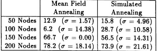
26.64)

Table 3.4: MFA vs. Simulated Annealing: Average Bin Imbalance

Mean Field Simulated Annealing Annealing 50 Nodes 12.9

(0-

=

1.57) 15.8

(0-

=

4.96) 100 Nodes 6.2

(0"

=

14.38) 28.7

(0"

=

10.58) 150 Nodes 66.7

(0"

==

0.00) 56.5

(0"

=

14.31) 200 Nodes 78.2

(0"

==

18.14) 73.9

(0-

=

21.61)

the exception of the 150 node graph, which seems to be deviant). However, mean field annealing found the solutions an average of 17 times faster than simulated annealing did. This large increase in execution speed without loss of solution quality is justification for the use of mean field annealing.

MFA Execution Time VB. Number of Nodes

In addition to being faster than simulated annealing, experimental results indicate that MFA execution time scales linearly with the number of nodes being partitioned. Figure 3.2 shows a plot of execution time (in seconds) vs. flow-graph size (in nodes), which demonstrates the linear behavior. This behavior implies that the number of iterations required for convergence is independent of the number of nodes and that the increase in execution time is due solely to extra nodes that must be processed in the inner loop of the MFA algorithm.

3.4

Scheduling

Once the flow-graph has been partitioned, the nodes assigned to each processor must be scheduled to eliminate as much waiting on other processors as possible. The algorithm used is the original PaLS scheduling algorithm ([Bou87]); it was simply recoded to use the new data formats of the modified PaLS system.

3.5

Code Generation

CHAPTER 3. MODIFICATIONS TO PALS 25

Time

(Seconds)

3000

. - - - . . , . - - - - r - - - . . . . , - - - - . . , - - - ,

2000

1000

O---Iooo..---...l"---...lL...---I"---_--'

o

1000

2000

3000

4000

5000

Number of Nodes

an enormous task.

However, most nsP's now have

C

compilers (especially new ones; see [PS88], [Fuc88], and [SK88]), and much work in writing custom code generators would be avoided by generating C code. Therefore, code generation is performed by convert-ing the IR code for each node into a C program. This approach has two advantages:

• it allows the code to be compiled and tested on the development platform

l

t uat is, a workstation), and

• it provides an easy way to make changes to the final code produced by PaLS (for example, hardware initialization code could easily be added to the front of the programs produced by PaLS).

Chapter

4

Trial Runs

The original PaLS system was tested by partitioning flow-graphs representing

• an IIR filter,

• an LMS (least mean squares) filter,

• and an adder tree.

The modified PaLS system was also tested using these flow-graphs, and the results (obtained by averaging the results of 25 partitionings for each flow-graph) were compared with those of the original system. The data for the original PaLS system are taken from [Bou87].

The results were compared using the ratio of the speed of the partitioned pro-gram, Sp, to the speed of the ideal partitioning, Si, where speed is the reciprocal of execution time. The ideal speed is given by

where

T = execution time

B

=

number of bins N = number of nodes

W n

=

weight of node n

Note that S, is calculated without regard to data dependencies and that it may be impossible to attain for some flow-graphs.

4.1

IIR Filter

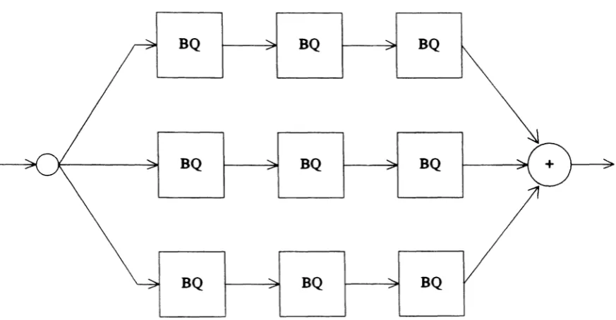
The modifications to PaLS were first tested by partitioning the parallel-cascade IIR filter shown in Figure 4.1. Table 4.1 lists the results obtained for both three and four processor partitions. In both cases, the modified PaLS system produced a partitioning that is faster than that produced by the original PaLS system.

Figure 4.1: Parallel-Cascade IIR Filter

Table 4.1: Results of Partitioning the IIR Filter

CHAPTER 4. TRIAL RUNS

4.2

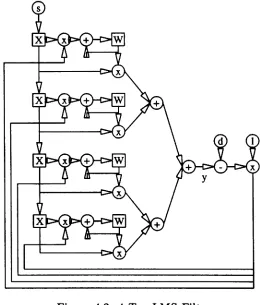
LMS Filter

29

PaLS was also tested by applying it to a 64-tap LMS filter. (A 4-tap filter is shown in Figure 4.2 for reference.) Table 4.2 shows the results for a four processor partition. For this filter, the new PaLS produced a partitioning that is slightly worse than

that of the original PaLS.

Figure 4.2: 4-Tap LMS Filter

Table 4.2: Results of Partitioning the LMS Filter

Bins ~_s· ~_s.

4.3

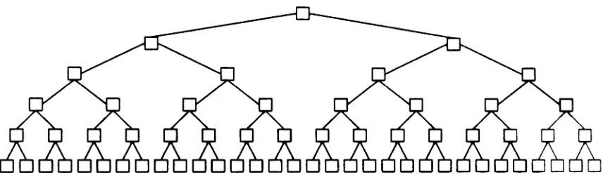
Adder Tree

As a final test, PaLS was applied to a 127 node adder tree; Figure 4.3 shows a 63 node tree, which contains one less "layer" than the 127 node tree. Table 4.3 lists the results for both three and four processor partitions. Surprisingly, the modified PaLS system produced better results for the irregular three partition case than for the very regular four partition case.

Figure 4.3: 63 Node Adder Tree

Table 4.3: Results of Partitioning the Adder Tree

Bins ~_s. ~_s·

3 =- 0.86

±

0.04

Chapter

5

Discussion and Further Work

The goal of the original PaLS system was to aid the design of networks of a custom DSP by automatically parallelizing signal processing algorithms. This system was modified with two goals in mind:

• to make PaLS as independent of the target processor as possible and

• to make PaLS easier to use.

A subgoal was to improve performance of the system, if possible, by improving the execution time of the partitioner.

A number of modifications were made to achieve the above goals. These changes include:

• use of a conventional programming language to specify algorithms,

• removal of dependencies on the custom DSP designed by Dr. Van den Bout,

• provisions to allow nodes to represent non-atomic operations,

• use of mean field annealing as the partitioning algorithm, and

• generation of C programs for each processor in the network.

5.1

The DFC Language

The DFC language is intended to make PaLS easier to use by providing an interface to PaLS that is more conventional and less cumbersome than a graphical editor.

5.1.1

Discussion of DFC

DFC achieves the goal of increasing the ease of use of PaLS by using a common programming language (C) as a vehicle for specifying algorithms. This has several advantages:

• there is no dependence on having a graphical editor that can generate flow-graphs in a format that PaLS can use

• C is a common language and is likely to be known by those using PaLS

• libraries of commonly used functions can be created

• standard UNIX programming utilities (such as make and ar) can be used.

There are a number of useful operations that are not present in DFC (see below); however, these operations can be implemented by making a function call. If the IR linker encounters a function call but does not have the body of that function available, it will leave the call in the linked output; during code generation, the IR to C converter will put a corresponding C function call in the C program. Therefore,

to implement a special operation in DFC:

1. Put a function call representing the operation in the DFC program.

2. Compile and link the DFC program without providing a definition for the function.

CHAPTER 5. DISCUSSION AND FURTHER WORK 33

4. The C code contains function calls corresponding to the calls made in the DFC program. The special operation can then be implemented by writing

the appropriate C function for each call.

5.1.2

Further Work on DFC

The DFC language can be improved in several ways, and these improvements will necessitate changes in other parts of the system. For example, the changes listed below will require substantial modification to the IR optimizer and partitioner; they might also require modifications to the linker and IR to C translator.

Additions to DFC

There are several additions that can be made to DFC to improve its usefulness for writing DSP programs and for writing programs in general.

Vector Operations. Many DSP algorithms include such vector operations such as dot product or

1

==

B

+

«c.

where

1,

B,

and

C

are vectors and a is a scalar; most digital signal processors have hardware support for these operations. Therefore, a vector notation would be useful in DFC because it would allow a more natural expression of DSP algorithms by programmers and it would allow the compiler to easily take advantage of hardware vector support.

Type Conversions. A method for explicit conversion between data types would probably be useful.

Enhancements to the

m

Optimizer

The IR optimizer can be enhanced by adding several more optimizations to those it already performs. Currently, the optimizer does constant folding, dead code elimi-nation, and copy propagation; it should be modified to do common sub-expression elimination. It could also do strength reduction, but this is not as important be-cause most DSP algorithms avoid division and most digital signal processors do addition, multiplication, and subtraction in a single cycle.

If iterative and conditional constructs are added to DFC, the optimizer will have to be modified. It will have to detect loop invariants, and it will have to take basic blocks into account (all optimizations are currently performed globally).

5.2

Partitioning

By replacing simulated annealing with mean field annealing, the time required to partition a flow-graph has been cut by an order of magnitude (Section 3.3.2) without reducing the quality of the solutions found. However, the method for determining the repulsion factor was found to be inaccurate, and the partitions generated for

random flow-graphs varied widely in quality.

In Section 3.3.1, the repulsion factor was given as

r

=

N-1

CHAPTER 5. DISCUSSION AND FURTHER WORK 35

in a single node. This behavior indicates that as the number of partitions increases, the repulsion factor must also increase. The exact relationship of the repulsion factor to the number of partitions needs further investigation.

[Ack82]

[Fuc88]

William B. Ackerman, "Data Flow Languages", IEEE Computer, Febru-ary 1982, pp. 15-25.

Michael L. Fuccio, ei. al., "The DSP32C: AT&T's Second-Generation Floating-Point Digital Signal Processor", IEEE Micro, December 1988, pp. 30-48.

[GBB86] Paul Le Guernic, Albert Benveniste, Patricia Boumai, and Thierry Gau-tier, "SIGNAL -AData Flow-Oriented Language for Signal Processing" , IEEE Transactions on Acou~tic~, Speech, and Signal Processinq, April 1986, pp. 362-374.

[KR78]

[Kir83]

[PS88]

[PE88]

Brian W. Kernighan and Dennis M. Ritchie, The C Programming

Lan-guage, Prentice-Hall, 1978.

S. Kirkpatrick, C. D. Gelatt, and M. P. Vecchi, "Optimization by Sim-ulated Annealing", Science, May 13, 1983, pp. 671-680.

Panos Papamichalis and Ray Simar, "The TMS320C30 Floating-Point Digital Signal Processor", IEEE Micro, December 1988, pp.13-29.

Ira PoW and Daniel Edelson, "Ato Z: CLanguage Shortcomings",

Com-puter Language, Vol. 13, No.2, 1988, pp.51-64.

BIBLIOGRAPHY

37

[SK88]

[Bou87]

[Bou88]

[Bou89]

Guy R. L. Sohie and Kevin L. Kloker, "A Digital Signal Processor with

IEEE Floating-Point Arithmetic", IEEE Micro, December 1988, pp.

49-67.

David E. Van den Bout, A Digital Signal Processor and Programming S'II,tem for Parallel Signal Processinq, Ph.D. dissertation, North Car-olina State University, 1987.

David E. Van den Bout and Thomas K. Miller III, "Graph Partitioning Using Annealed Neural Networks", North Carolina State University, 1988. Submitted to IEEE Transactions on Circuit, and S'II,teml.

DFC Reference Manual

This appendix provides a reference manual describing the DFC programming lan-guage. DFC is basically a subset of C with a few additions and restrictions for DSP programming and for partitioning. The manual follows that in [KR78].

A.I

Lexical Conventions

A DFC program consists of ideniifiers, keywordA, constants, operators, and separa .. tors. White space (including comments) is ignored except when used to separate any of the above items.

A.I.I

Comments

A comment starts with the characters

r:

and ends with • /. Comments cannot be

nested.

A.l.2

Identifiers

An identifier consists of a letter or underscore followed by zero or more letters,

APPENDIX A. DFC REFERENCE MANUAL

A.l.3

Reserved Words

The following seven identifiers are reserved:

39

float for input int

main output return

The word for is unimplemented but reserved for future use.

A.l.4

Constants

DFC allows two types of constants: integer and floating point. DFC makes no guarantees whatsoever concerning the hardware representation of numbers.

Integer Constants

There are three types of integer constants: decimal, hexadecimal, and binary. A decimal constant is a sequence of one or more digits; a hexadecimal constant consists of Ox or OX followed by one or more hex digits; and a binary constant consists of Ob or OB followed by one or more binary digits. The digits are '0'..'9'; the hex digits are '0'..'9' and 'a'..'f'; and the binary digits are '0' and '1'.

Floating Constants

All floating point constants are in decimal and may take one of the following forms:

• One or more digits followed by an exponent.

• One or more digits followed by a decimal point.

• One or more digits followed by a decimal point followed by one or more digits.

• One or more digits followed by a decimal point followed by an exponent.

• One or more digits followed by a decimal point followed by one or more digits followed by an exponent.

• A decimal point followed by one or more digits followed by an exponent.

An exponent consists of an e or E followed by an optional sign

('+'

or '-') followed by one or more digits.

A.2

Variables

DFC supports two types of variables: Int and float. All variables are local to the "function in which they are defined (see below). Storage for variables is meant to match the underlying processor; therefore, DFC makes no guarantees about the

representations of int's and float's.

A.3

Expressions

An expression is a sequence of operators and operands. Operands are identifiers,

constants, or expressions surrounded by parentheses.

A.3.1

Operators

The operators in DFC are as follows:

{ezpreAAion} Group the entire expression into one node (aAupernode)I

(ezpre&Alon) Change the precedence of expression.

-ezpressson Negate (two's complement) the operand.

expression One's complement of the operand. Iexpression Absolute value of the operand.

@ezpre.,.,ion Delayed value of the operand.

APPENDIX A. DFC REFERENCE MANUAL 41

expression &; expression expression I expression

output(id,con~tant)

expression > ezpressuni

Output the value of the identifier to the specified output port.

Integer or floating point multiplication. Integer or floating point division. Integer modulus.

Integer or floating point addition. Integer or floating point subtraction.

Shift the left integer operand left by the number of bit positions specified by the right integer operand.

Shift the left integer operand right by the number of bit positions specified by the right integer operand.

Rotate the left integer operand left by the number of bit positions specified by the right integer operand.

Rotate the left integer operand right by the number of bit positions specified by the right integer operand.

Bitwise AND of the two integer operands.

Bitwise exclusive OR of the two integer operands. Bitwise OR of the two integer operands.

expression

.

.

ezpre"lon - ezpreA,,,on

expression

<

ezpressum

expression

expression • expression ezpression / expression ezpression % expression expression

+

ezpressioti

expression >

>

expression expression

<<

expression

A.3.2

Precedence Rules

The precedence of the expression operators is shown in Figure A.I, where higher precedence operators are on top. The order of evaluation of expressions is unspeci-fled, except that the precedence and associativity rules will be obeyed.

A.4

Declarations

Declarations are of the form

type-name identifier-lilt;

Table A.I: Operator Precedence

I

Associativity

I

Operators

{} () -

-

I @ input output Right to left

* / % Left to right

+ -

Left to right

<

>

«

»

Left to right

& Left to right

....

Left to right

I Left to right

A.5

Statements

DFC has three types of statements: declarations (see above), assignments, and

compiler control lines.

Assignment statements are of the form

identifier

==

expression ;

DFC uses the single assignment rule; therefore, an identifier can only appear as the

target of an assignment once.

DFC uses the C preprocessor for including files, macros, and conditional

com-pilation. See the description in [KR78].

A.6

Functions

DFC uses the same syntax as C ([KR78]) for function declarations, except that the

function must be explicitly typed. The syntax is

typeJpec Junc_name ( parameter" ) typeJpec parameiers ;

APPENDIX A. DFC REFERENCE MANUAL

return ( return_val) ;

}

43

All parameters are passed by value, and the result is returned with the return statement. The argument of return can only be an identifier of the same type as the function, and return has to be the last statement of the function.

A.7

Scope Rules

maIn program

A DFC program is made up of a list of function declarations followed by the body of the main program, which is the main function as in C:

main()

{

}

All function names are globally visible. If a function is used before it has been defined, then it is assumed to be of type int; if the function is of type float, the scope in which it is used should contain the declaration

float func_name();

There are no other global names; all variables declared in a function are local to that function.

These scope rules permit programs to be spread across several files, which can each be compiled separately. When the resulting modules are linked, the linker checks that the types of the actual and formal parameters match.

A.8

A DFC Grammar

,-,

.

_,

,-,

.

_,

, ,.

_,

'i'j '%' ;

,."

. ,

'I'·

. ,

'.'

,

,.

.

,

,

,\,, ",

,

'*' ;

1I'; ",; 'G'j , c, 'I'j

,.,

_,

.

_,

, ,J .,

,tI, ._, ,-,_-

.

_,

,

(

,

; ,)

,

;

,

[,; ,]

,

; ,{,; ,},; ,<, ; ,>, ;

'+' ;

,-,

.

,

'a', 'c' ..'d', 'f', '1', 'C' .. 'D', 'F'; 'b', 'B'j

'e', 'E';

'x', ' I ' ;

'G' .. 'L', 'H' .. 'W', 'T', 'Z', 'g' ..'l', 'm' .. 'v', 's>, 'z';

'2' .. '9';

'0' ;

, i : ;

, ,.

_{- ,}

,

,.

_,

9; 10;

1 .. 8,11 .. 31,127;

[20,30] {2} 'FLOAT',

[20,20] 'FOR',

[20,20] 'INPUT' ,

APPENDIX A. DFC REFERENCE MANUAL

%TOKENS

Letter

=

Bletter, Eletter, BexLetter, Iletter, OtherLetterj

~IG.ORE (Blank{TOSS}, Linefeed{TOSS}, Tab{TOSS})+,

(SlashCh{TOSS}.StarCh{TOSS}.(IOT(StarCh){TOSS}, StarCh{TOSS}+.IOT(StarCh,SI.ahCh){TOSS}) •. StarCh{TOSS}+.SlashCh{TOSS})j

I. Decimal, Hex, Binary, Floating, a String constants . •1

Digit

=

Zero, One, IzDigitj

BexDigit

=

BexLetter, Bletter, Eletter, Digitj HexMark = Zero.Iletterj

BinMark

=

Zero.Bletter;

%TOKEI constant [20,20] {1} = Digit+j

~TOKEI constant [20,20] {2}

=

BexMark.(BexDigit)+;

%TOKEN constant [20,20] {3}

=

BinMark.(Zero,One)+j

DottedDigits = (Digit+.DotCh),(Digit+.DotCh.Digit+),(DotCh.Digit+)j Exponent = Eletter.(PlusCh, MinusCh, EPSILON).Digit+j

%TOKEB constant [20,20] {4}

=

Digit+.Exponent,(DottedDigits.(Exponent,EPSILOI»j loDQCh: lOT (NonPrint, Tab, Linefeed, DoubleQuote)j

%TOKER constant [20,20] {6} : DoubleQuote{TOSS}.NoDQCh•. DoubleQuote{TOSS}j %TOKER ":It [20,20] : EquaICh{TOSS};

%TOKEN II(It [16,14]

=

LParenCh{TOSS};

%TOKER ")" [16,16] ; RParenCh{TOSS};

%TOKEN [20,20] TildeCh{TOSS};

%TOKEN ,,_It [20,20]

=

MinusCh{TOSS}; %TOKEN ,,+It [20,20]

=

PlusCh{TOSS}; %TOKEN "." [20,20] StarCh{TOSS}j %TOKEN _"I" [20,20]

=

SlashCh{TOSS}; %TOKEI "%,, [20,20]

=

PercentCh{TOSS}; %TOKEN ,,<It [20,20]

=

LTCh{TOSS}; %TOKEN ">,, [20,20]

=

GTCh{TOSS};

%TOKER ,,«~It _[20,20]

=

_{LTCh{TOSS}.LTCh{TOSS};}

%TOKEB "»,, [20,20]

=

GTCh{TOSS}.GTCh{TOSS}; %TOKEI "t" [20,20]

=

lmpCh{TOSS}j

%TOKEB "...." [20,20]

=

CaretCh{TOSS}j

%TOKEI "I" [20,20]

=

BarCh{TOSS}; %TOKEI _",_" [16,16] CommaCh{TOSS}; %TOKEI ".It, [10,30]

=

SemiCh{TOSS}j %TOKEI It{" [16,16]

=

LBraceCh{TOSS}; %TOKEI "}" [16,16]

=

RBraceCh{TOSS}; %TOKEI Delay [16,16]

=

ltChar{TOSS}; %TOKEI preline [30,30] : Pound{TOSS}; FirstCh : Letter, Underscorej

FollovCh = Letter, Underscore, Digit; %TOKEI id [16,17] = FirstCh.(FollovCh).

%EICEPT float for

input

int main output return

[16,30] {1} 'IMT',

[20,20] 'MAIN', [20,20] 'OUTPUT' , [20,20] 'RETURN';

~production8

<prog> ::= <function list>

<function list> .. - <function> <function list> ; .. - main "(" II)" "{" <body> "}" i

.. - preline constant constant <function list>;

<function> ::= <decl type> id "(" <formals> ")" <formal decls> <fnnc body>

<formals> ::= id <more formals>

• • - J

<more formals> II,II _{id <more formals>}

<formal decls> .. - <decl type> id <formal list> I f . 1 I

J <formal decls>

<formal list> II,II _{id <formal list>}

• • - J

<frmc body> ::= "{" <body> return "(" id ")" "i" I I } "

<body> ::= <decl list> <stmt list>;

<decl list> ::= <decl> <decl list> ;

• • - J

<decl> ::= <decl type> id <decl follow> <decl follow> .. - "(" ")" <var list> "i"

.. - <var list> "i"

<decl type> int

float

<vax list> ::= "," id <var list follow> j

::= ;

<var list follow> "(" ")" <var list> i

<var list> ;

<8tmt list> ::= <stmt> <stmt list>

: :=

<stmt>

<expr> : :=

preline constant constant id "=" <expr> "i"

.,.,1 • J ,

APPENDIX A. DFC REFERENCE MANUAL

<I bexpr2*> ::= "1" <b expr2> <I bexpr2*>

..

- ,

<b expr2> ::= <b expr3> <~ bexpr3*> ;

<... bexpr3*> ::= I I - I I <b expr3> <~ bexpr3*>

::= ;

<b expr3> ::= <s expr> <i rexpr*> ;

<i rexpr*> ::= "i" <s expr> <i rexpr*>

..-

,

<s expr> ::= <arith expr> <shift arexpr*>

<shift arexpr*> .. - ,,<It <ari th expr> <shift arexpr*> ; .. - ">" <arith expr> <shift arexpr*> ; .. - ,,«~It <axith expr> <shift arexpr*>

.. - "»" <arith expr> <shift arexpr*>

<arith expr> ::= <term> <+ term.> ; <+ term*> .. - "+" <term> <+ term.>

::= ,,_It <term> <+ term.>

..

-

,

<term>

..

-

<primary> <* prim.>

<. prim*>

·

.-

"." <primary> <* prim.>

·

.-

"ilt <primary> <* prim*>

·

.-

n%" <primary> <. prim*>

·.-<primary>

·

.-

"(It <expr> ")" ;

·

.-

It{" <expr> It}" ;

·

.-

"_" <primary>

·

.-

<primary>

·

.-

"I" <primary>

·

.-

Delay <primary>

·

.-

constant ;

·

.-

id <structure>

·.-

input II(It _{constant ")" ;}

·

.-

output n(" _{id "," constant ")"}

<structure> .. - "(n <expr list> ")"

..

-

..-<expr li.t> ::= ..-<expr> <, expr list>

47

IR Reference Manual

The IR (Intermediate Representation) is a list of expressions that represents an algorithm in a form that can be easily read by a number of different tools. This chapter gives a description of the IR.

B.l

Node Names

Each statement (see below) in an IR program represents a computational node in a flow-graph; the node number is therefore used as the name of the statement. To distinguish constants from node names, constants are preceded by a single quote

(').

B.2

The main Section

The main section of an IR program is a sequence of statements preceeded by the word main and followed by the word end:

rnam

statement-list

end

APPENDIX B. IR REFERENCE MANUAL

49

B.3

Function Definitions

A function definition consist s of a header, a list of type specifiers, a st atement list,

and a return specifier.

A function header is of the form

function [unc.suune type ( parameter_li,t )

where [unc.natne is the alphanumeric name of the function, type is a integer spec-ifying the data type returned by the function, and parameter.lisi is a list of node names separated by spaces.

A type specifier has the form

type parameter.name data_type

where parameter.name is one of the node names in the parameter list of the function header, and data_type is the data type of that parameter. The type specifiers do not have to be in the same order as the correspondings parameters in the parameter list.

A return specifier has the form

ret return.node

where return.node is the node whose value is the result of the function.

B.4

IR Statements

An IR statement is of the form

(==

node:type ezpre"ion)

B.4.1

Expressions

An IR expression is either a node name, an integer or floating-point constant pre-ceded by a single quote, or a subexpression. There are three forms of subexpressions; the form expressing a function call is

(call name weight ( argument~ )) the form using unary operators is

(operator ezpre3sion)

and the form using binary operators is

(operator expression ezpre33ion)

where expression is an IR expression as defined above. This definition allows ex-pressions to be nested to any depth.

B.4.2

Function Calls

A function call has the form

(call name weight ( arqumenis ))

where name is the alphanumeric name of the function being called, weight is the computational weight of the function being called, and argumentl is the optional

argument list.

Each argument is of the form

( type eepression )

where type is the data type of the argument, and ezpressioti is the actual argument. An argument expression can be any of the expression types listed above, except

APPENDIX B. IR REFERENCE MANUAL

Table B.l: IR Operators

Operation Number of Operands Operand Types Result

+ op1 op2 2 float/int op1 plus op2

- op1 op2 2 float/int op1 minus op2

• op1 op2 2 float/int op1multiplied by op2

/ op1 op2 2 float/int op1 divided by op2

I: op1 op2 2 int op1 AND op2

I op1 op2 2 int op1 OR op2

- op1 op2 2 int op1 XOR op2

<op1 op2 2 int op1 shifted left op2 times

>op1 op2 2 int op1 shifted right op2 times

{ op1 op2 2 int op1 rotated left op2 times

} op1 op2 2 int op1 rotated right op2 times

a op1 1 float/int absolute value of op1

n op1 1 float./Int negation of op1

., op1 1 int l's complement of op1

B.4.3

Operators

51

There are 11 pre-defined binary operators and 4 pre-defined unary operators; Ta-ble B.l gives a list of the operators.

B.4.4

Input/Output

There are four special types of operators for doing input/output that may be used anywhere a normal subexpression may be used. The I/O operators are

• I Iconsi

Inputs a value from the input port specified by the integer constant Iconsi

• 0 ezpression Iconsi

• t expression

Transmits the value of expression to another processor

• r node

Receives a transmitted value from the node node (which is expected, but not required, to be a transmit node)

B.5

IR Grammar

The following is a description of the IR format suitable for use with the cgen scanner / parser generator:

%OPTIONS list_vocab list_bn1 list_scan scan_table parse_table optimize_time optimiz8_dfa %TERMIIALS OtherLetter ALetter ILet'ter RLetter SLetter TLetter ULetter Digit PluaCh Minu8Ch StarCh SlashCh impersandCh BarCh CaretCh itCh TildeCh LingleCh RingleCh

- 'b' ..'m', 'o' .. 'q', 'v' .. 'z', 'B' .. 'M', 'O' ..'Q', 'V' .. 'Z'

= 'a), 'A'

'n', )1'

'r', 'B'

= '8', '5'

=

't', 'T'

=

'u',

'U'

= '0' .. '9'

=

'+ '

=

,-,

=

'.'

=

'I'

=

't'

=

,

I'

APPENDIX B. IR REFERENCE MANUAL

EqualCh

= '='

;

QuoteCh

=

'" ,

;

LBraceCh

=

,{

,

RBraceCh

=

,},

LParenCh

=

,

(,

RParenCh

=

,

)

,

SemiCh

=

,.

,

,

Underscore

=

,

,

DotCh

=

,

,

ColonCh

=

J : J

Illegal _'I' 'c,

,

[,, _'\',

'.'

, ,~

,

'''' ,]

,

, '%' , 'I' ,

,

J .

, , , ,

Blank

, ,

.

,

Tab

=

9;

Linefeed

=

10;

NonPrint

=

1 .. 8, 11 .. 31, 127;

%TOKENS

Letter

=

ALetter, BLetter, SLetter, RLetter, TLetter, ULetter, OtherLetterj

%IGNORE (Blank{TOSS}, Tab{TOSS}, Linefeed{TOSS})+ j

%TOKEN IConst [2,2] {O} = QuoteCh{TOSS}.(MinusCh,EPSILOB).Digit+j

%TOKEN FConst [2,2] {1}

=

QuoteCh{TOSS}.(MinusCh,EPSILOI).Digit+.DotCh.Digit*;

%TOKEN Comment [2,2] {O} = SemiCh{TOSS}.(NOT(Linefeed){TOSS})*.Linefeed{TOSS}

%TOKEN Number [2,2] {O}

=

Digit+;

FollovCh

=

Letter, Underscore, Digit

%TOKEN Id [20,20]

=

Letter. (FollovCh)

*

%EICEPT

"a" [20,20] {10} _'.A.' ,

abs [20,20] {10} 'ABS' , call [20,20] {31} 'CALL' , end [20,20] 'END' ,

function [20,20] 'FUNCTION' ,

input _{[20,20] {11} '1 '} ,

load [20,20] {12} 'LINK_LOAD' ,

unload [20,20] {16} 'LIIK_UNLOAD' ,

main [20,20] 'MAIN' ,

"n" [20,20] {13} '11 ' ,

neg [20,20] {13} 'lEG' ,

output [20,20] {14} _'0' ,

"r" [20,20] {16} 'R' ,

ret [20,20] 'RET' ,

"s" [20,20] {le} _'5' ,

"t" [20,20] {12} 'T' ,

type [20,20] 'TYPE' ,

"u" [20,20] {17}

'u'

,

store [20,20] {1e} 'Z_STORE' ,

update [20,20] {17} 'Z_UPDATE'

%TOKEN "+" [20,20] {18}

=

PlusCh{TOSS} j

%TOKEN "_" [20,20] {19}

=

MinusCh{TOSS} ;

%TOKEN

...

_{[20,20] {20}}

=

_{StarCh{TOSS} ;}

%TOKEN ../

..

_{[20,20] {21} SlashCh{TOSS} ;}

%TOKEN

"a"

_[20,20] {22}

=

_{AmpersandCh{TOSS}}

%TOKEH

"',,

[20,20] {23}

=

BarCh{TOSS} ;

%TOKER

...

[20,20] {24}

=

Caret Ch{TOSS}

%TOKEN

"'"

[20,20] {26}

=

itCh{TOSS} ;

%TOKEN ..-" [20,20] {26}

=

TildeCh{TOSS}

%TOKEB ..<" [20,20] {27}

=

UngleCh{TOSS}

%TOKEB ">,, [20,20] {28}

=

lllngleCh{TOSS}

%TOKEI ,,{.. [20,20] {29}

=

LBraceCh{TOSS}

%TOKEN "}" [20,20] {30} = RBraceCh{TOSS}

%TOKEW "=" [20 t2O] {40} = EquaICh{TOSS} ;

%TOKEN "(II _{[20,20] {41} LParenCh{TOSS} ;}

%TOKEN ")11 _{[20,20] {42} = RParenCh{TOSS} ;}

%TOKEN II • .,

[20,20] {43} = ColonCh{TOSS} ;

%productions

<program> ::= <block_list> ;

<block> <block_list>

<block> main <statement_list> end ;

function Id lumber .,( .. <pararn_Iist> II)" <type_list> <statement_list>

ret lumber ;

lumber <param_Iist> : :=

type lumber Number <type_list>

<statement_list> <statement> <statement_list>

<statement> ..(.. "='1 lumber ... " lumber <expression> ")II

Comment

<expression> : :=

: := 11(" <operation> IConat FConat lumber ")"

<operation>

·

.-

"+" <expression> <expression>

: := It_" <expre •• ion> <expression>

·

.-

"." <expression> <expression>

APPENDIX B. IR REFERENCE MANUAL

·

.-

11"'11 _{<expression> <expression>}

·

.-

"~" <expression>

·

.-

I I - I I _<expression>

·

.-

"<" <expression> <expression>

·

.-

">,, <expression> <expression>

·

.-

"{" <expression> <expres.ion>

·

.-

"},, _{<expression> <expression>}

·

.-

abs <expression>

·

.-

"a'i <expression>

·

.-

neg <expression>

·

.-

lin" <expression>

·

.-

load <expression>

·

.-

"t" <expression>

·

.-

unload <expression>

·

.-

"r" <expression>

·.-

store <expression>

·

.-

"s" <expression>

·

.-

update <expression>

·

.-

"U" <expression>

·

.-

<I/O> ;

·

.-

<call> ;

<call> ::= call Id Number "(" <arguments> ")" ;

<arguments> .. - "(" lumber <expression> If)" <arguments>

<I/O> .. - input IConst

.. - output <expression> IConst

PaLS Programs

The following sections describe the programs that make up the PaLS system.

c.r

DCC - Compiler/Linker/Optimizer Control

This program provides a single control point for the DFC compiler, the IR linker, and the IR optimizer. The program is invoked by

dec [-c] [-01]

[-0

filename] file~

where the options have the following meanings:

-c

-0 filename

-01

The link phase is suppressed.

The compiled, linked result is written to filename.

Use optimization level 1. In this level, the optimizer will try to reduce the number of statements by propagating statements that are only used once.

APPENDIX C. PALS PROGRAMS 57

C.2

DFC - DFC Compiler

The DFC compiler is invoked as follows:

dfc source.file IR_file

The DFC source program in source.file is compiled into IR format, and the IR

output is placed in IR_file.

C.3

OPT - IR Optimizer

The optimizer performs various optimizations on programs in IR format. It is run

by typing

opt opt.levelinput_file output_file

where opt.level is the optimization level (see below), input_file contains the IR to optimize, and output_file is the optimized IR.

The optimizer performs several types of optimizations:

• constant folding

• dead code elimination

• copy propagation

Dead code elimination removes all nodes whose results are never used. However, function calls and I/O statements are not removed so that any side effects are preserved.

(10:0 12)

were found, all occurrences of 10 would be replaced by 12. This optimization is performed in levels 0 and 1.

Second, if the result of a statement is only used once, the statement name at the use is replaced with the statement's expression. For example, if the sequence

(23:0

(+

14 15))

(88:0

(*

23 18))

occurs and the only use of statement 23 is in statement 88, then statement 88 will be replaced by

(88:0

(* (+

14 15) 18))

However, if a statement contains I/O, it will not be propagated to ensure that the I/O operations are performed in the originally specified order. This optimization is only performed in level 1.

Delays are implemented by using a value before it is defined; for example,

a

=

b; b = value

assigns the delayed value of b to 8. Therefore, forward references (that is, the use

of b in a

=

b;) and backward definitions (that is, the assignment of a value to b

APPENDIX C. PALS PROGRAMS 59

C.4

LNK - IR Linker

-w

-0 filename

The IR linker resolves all function calls; it is invoked by

Ink [option.9] IR_file.9

where IR_file.9 represents one or more IR files. The options to Ink are

The linked result is written to filename.

Function calls are not expanded (see below); however, the function weights in the calls are updated to be the actual weight of the function.

WARNING!!! The IR files produced by the DFC compiler MUST be run through the optimizer before they can be linked.

The linker reads all of the IR files and resolves all function calls found. Calls are resolved by checking that the types of the actual and formal parameters match and then inlining the body of the function at the point of the call. Recursive functions are not allowed, but no checks are made.

If the -w option is specified, the functions will not be inlined. However, the weight of each function will be computed and placed into each call of the function. With this option, recursive functions can be linked.

If one of the IR files contains the main block, only the expanded main block is written to the output file; otherwise, all of the expanded functions are output. The output will probably contain redundant assignments and should be optimized.

C.5

PAS - Partitioner Control

pas bins IR_file

where bins is the number of processors to partition into and IR_file is the IR program to partition. PAS runs the renumberer, partitioner (with a set of default control parameters), and scheduler to produce an IR program for each of the processors. It then converts each of the IR programs into a C program.

C.6

RNO - IR Renumberer

The IR renumberer prepares IR files for partitioning and is invoked by

rno in_file out_file

The renumberer reads in a section that contains only a main section and renum-bers the statements so that the first statement is numbered 0 and the following statements are number consecutively. The renumberer also performs the same level

o

optimizations that are performed by the optimizer.

C.7

MFA - Partitioner

The partitioner reads in a linkedIR f