STRAIN HARDENING AND TRIAXIALITY EFFECTS ON THE
ηηηη
FACTOR
Philippe Gilles1, Vincent Robin2, and Emmanuelle Debourdeaux3
1
AREVA Fellow, Expert in Mechanics and Materials, Paris La Défense, France ([email protected])
2
AREVA expert in manufacturing process, AREVA NP, Lyon, France
3
ENPC student, Champs sur Marne, France
ABSTRACT
The most widely used approach to assess fast fracture is based on the crack driving force J. The criteria for crack initiation and stable growth compare J to a fracture resistance parameter JIc or a
J-Resistance curve. The determination of fracture resistance parameters is based of an estimate of the crack driving force J as a proportion of the plastic work per unit ligament area. This proportion is given by the so called η factor, which is a function of the cracked structure and valid only for deep cracks.
It is concluded that the η factor could be extended to shorter cracks, by accounting for strain hardening effects. The paper provides for CC(T) and SE(B) specimens, a constraint criterion giving the crack size limit as a function of the hardening exponent over which strain hardening effects may be neglected and a general formula for the CC(T) specimen. However, it should be kept in mind that the loss of constraint corresponds to a loss of J significance as a fracture criterion.
INTRODUCTION
Elasto-plastic fracture mechanics is commonly used for defect assessments in Nuclear Industry. Most of the approaches are based on the crack driving force J which is compared to a fracture resistance parameter. This fracture resistance parameter cannot be measured directly, but requires as well as J engineering formulae or Finite Element computations. This paper address two issues: the validity of the
η factor approach (Turner, 1980) used to derive fracture resistance from test records and the determination of hardening dependent η factor with extended validity limits. The approach uses the consistency of η factor formulae with the GE-EPRI J estimation scheme (Kumar, 1981).
DEFINITION OF THE ETA FACTOR APPROACH
The crack driving force J is widely used for fracture toughness measurements mainly because it covers small and large scale yielding. However this parameter cannot be measured directly as opposite to the CTOD parameter. Measuring the fracture toughness parameter JIc using the integral definition would
be possible only in plane stress conditions, which would be very inaccurate regarding specimen geometries. Therefore the definition of J as the energy release rate in non-linear elasticity has been used.
In small scale yielding, where the specimen may be modeled in linear elasticity, J is related to the mode I Stress Intensity Factor (SIF) KI through the relation:
(
)
2I 2 e
K E
ν 1
J = − (1) Where the SIF is proportional to the applied stress and is non linearly
dependant of the crack size a: K=F(a/W)σappl
( )
Q πa enc appl
Z Q
σ = where Q is the load and
e nc
In non linear elasticity (Applicable to plasticity under strictly increasing loading) the energy release rate is expressed respectively under fixed grips conditions and constant load conditions as:
dq A Q J
0 q
q
∫
∂∂−
= (2a) dQ
A q J
Q Q
0
∫
∂∂= (2b)
The J parameter appears here as a derivative of the plastic work =−
∫
⋅q
0 p
dq Q
W .
Brief history of the ηηηη factor approach
The first experimental method for determining JIc in large scale yielding was published by Landes
and Begley (1972, 1979) and estimated J by deriving load-displacement curves for several specimens of identical type but with different crack lengths. Then energy-crack length curves were derived allowing obtaining the derivatives.
Considering deeply cracked specimens, where plasticity is confined in the ligament, Rice, Paris and Merkle (RPM, 1973) established that J could be obtained from a single load-displacement record. The expressions depend on the form of the relationship between the plastic displacement due to the crack and the load. The RPM approach relies on two key hypotheses:
1. Separation of elastic and plastic components of the displacement: the total displacement qt is the sum of the displacement obtained in the linear elastic case and the displacement corresponding to a pure plastic behavior : qt = qe + qp
2. A separability of the load displacement relationship: the load is the product of the ligament times a material behavior dependant function of a plastic displacement.
For the Central Crack panel in Tension (CC(T)) specimen and the Single Edge specimen in pure bending (SE(B)) the formulae for the deep crack solution JDC are respectively:
=
∫
pq
0 p p
DC 2 Qdq -Qq
2Bb 1 J
p
and =
∫
p
θ
0 p c p
DC Mdθ
Bb 2 J
Where B is the specimen thickness, 2b the ligament for the CC(T) and b for the SE(B) As shown in Figure 1 the area is different for the CC(T) and the SE(B).
D C
A
B
0 q
Q
D C
A
B
0 q
Q
Half plastic area associated to JpDC for the CC(T) Plastic area associated to JpDC for the SE(B)
Thus Jp is a product of a geometric factor ηp times the area (or a part of it) under the
load-displacement curve. p
S P p DC A b k B η J ⋅ ⋅
= , whereks = 2, η
p
= 1 for the CC(T) and ks = 1 , η
p
= 2 for the
SE(B).
From these results Sumpter and Turner (1976) proposed a general formula :
b k B A η b k B A η J J J S p p S e e p e ⋅ ⋅ ⋅ + ⋅ ⋅ ⋅ = + = Where a C C b ηe ∂ ∂
= is obtained from the elastic compliance C =Q/q. Such a presentation is
attractive, but some authors considered an average η factor
b k B A η J S t t ⋅ ⋅ ⋅
= which may be erroneous since
ηe
and ηp behave differently such as for the CC(T) specimen.
Triaxiality and material behaviour effects on the ηηηη factor
This paragraph examines the effect of the type of material constitutive law on the existence of the η factor as a purely geometric factor and the impact of stress triaxiality in front of the crack on the value of the η factor.
The load separability, a condition of existence of a purely geometric η factor
The RPM analysis demonstrated the existence of a purely geometric η factor on the basis of a property of separability of the load-displacement relationship. We define the separability of the load-displacement function by the following decomposition
( )
( )
= a g q F a f Q Where :f and g are functions of the geometry of the cracked structure symbolized by the crack size a and independent of material characteristics.
F is a function dependant of the material constitutive law. There are two types of separability functions:
The general case is the tensile specimen case analyzed by Rice and al. (1973). J is proportional to a particular part of the plastic work.
If the function g is independent of the crack geometry, then J is proportional to the plastic work. This corresponds to the case of the bending specimen. The study of Sharobeam and Landes (1991) considers only this type of separability and their load separation criterion is not general.
It may be easily shown that if f or g depends on material characteristics as in the GE-EPRI handbook (Kumar, 1981), then the η factor depends on the hardening law. We may propose for the existence of a hardening dependent η factor a more general statement:
For a purely plastic material obeying to a power hardening law n eq
eq σ
ε =κ ⋅ , Illiushin’s theorem states
that under radial loading the load-displacement relationship takes a similar form: qcp= C(a,n)Qn. The
plastic work is then p
c p c q 0 p
c Q q
1 n n = dq Q W p c ⋅ ⋅ +
=
∫
andTherefore
a C
C b ηp
∂ ∂ ⋅
= , which is positive since C increases with increasing crack length. As well as C,
η depends on the hardening exponent n. This will be illustrated later in this paper. Linear elasticity
The elastic work is the work recovered by elastic unloading (CDB area in Figure 1b). The
expression is therefore :
2 q Q dq Q W
0
e = ⋅ = ⋅
∫
q
. The load and displacement are related by the
compliance C: q=C⋅Q. The linearity of the behavior ensures the separability of the load-displacement
relationship. We have two expressions of Je : the Irwin’s expression :
(
)
2I2 e
K E
ν 1
J = − and
e 2
0 e
W A C C
1 2 Q A C dQ A
q
J ⋅
∂ ∂ = ⋅ ∂ ∂ = ∂
∂ =
∫
q q
. This gives
a C C b
ηe ∂ ∂
= and an expression of the compliance
as a function of the SIF (Turner, 1980).
We get :
∫
=
da a F
a F b η
2 2 e
where F is the Linear Elastic Fracture Mechanics (LEFM) shape factor
( )
Q πa σF(a/W)
K= appl .
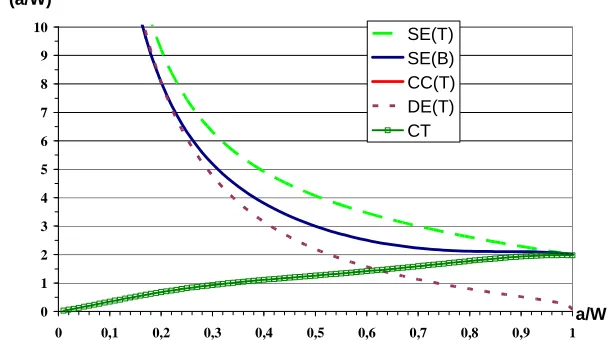
These functions are highly dependent on a/W as shown in Figure 2. In practical application the elastic compliance corresponding to the uncracked specimen attenuates greatly the variation range of the η factor in the a/W < 0.5 crack range. The shape factors are those of the Tada handbook (Tada, 2000).
0 1 2 3 4 5 6 7 8 9 10
0 0,1 0,2 0,3 0,4 0,5 0,6 0,7 0,8 0,9 1
a/W ηηηηe
(a/W)
SE(T) SE(B) CC(T) DE(T) CT
Figure 2: Elastic η factors due to crack for several specimens
Rigid Perfectly Plastic constitutive law
For a Rigid Perfectly Plastic material, the load is constant and equal to the limit load QL, thus
independent of the displacement, and the plastic work is simply given by the product QL *q . Under
simple loading, the limit load QL takes the general form:
p L_nc c 0
0L_c σ µ Z
Q = , where σ0 is the yield limit,
p L_nc
Z is the plastic modulus of the uncracked section and µc a crack factor which is the product of a
q Q da dµ µ 1 B 1 B q Z σ da dµ q da B dQ dq A Q J L c c p L_nc 0 c L 0 ⋅ ⋅ = ⋅ ⋅ = ⋅ ⋅ = ∂ ∂ − =
∫
q qWe note X = a/W the relative half crack length, W being the half specimen width, thus b=W⋅
(
1-X)
.The RPP
η
pL factor is :(
)
+ ⋅ − = − = X d µ d µ 1 X d µ d µ 1 X -1 X d Q d Q X -1 η t t r r L L p L
For the CC(T) specimen, the triaxiality factor is equal to unity : Q0L_c =kVM⋅σ0⋅µc⋅ZpL_nc
where
3 2
kVM = in plane strain or 1 in plane stress, µc ≡µr =1-X,
We have therefore
η
pL=
1
.For the SE(B) specimen, the limit load expression is the same with µr =
(
1-X)
2 and a triaxialityfactor which depends strongly on X for X < 0,3. The η factor takes the form:
X d µ d µ X -1 2 η t t p
L = +
For deep cracks (X > XS) µt =1.263 and
η
2
p L
=
For shallow cracks (X < XS), the limit load decrease for decreasing crack length. One of the best
estimates has been obtained by Wu (1990) using Finite Element. The shallow crack size XS equal
0,317, the fitted triaxiality factor is given by µt =2⋅
(
0.4978+0.8427⋅Xaw-1.328⋅X)
We obtain the formula :
(
)
2 p L X 1.328 -Xaw 0.8427 + 0.4978 X 2.656 -0.8427 X -1 2 η ⋅ ⋅ ⋅ − =
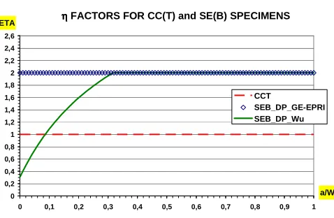
Figure 3 compares the η factor solutions for CC(T) and SE(B).
ηηηη FACTORS FOR CC(T) and SE(B) SPECIMENS
0 0,2 0,4 0,6 0,8 1 1,2 1,4 1,6 1,8 2 2,2 2,4 2,6
0 0,1 0,2 0,3 0,4 0,5 0,6 0,7 0,8 0,9 1
a/W ETA
CCT
SEB_DP_GE-EPRI SEB_DP_Wu
Figure 3: Rigid Perfectly Plastic η factors for CC(T) and SE(B)
For shallow cracked SE(B) the stress triaxiality decreases with decreasing crack length, and reduces the η factor value.
For the CC(T) specimen,
=
∫
pq
0 p p
DC 2 Qdq -Qq
2Bb 1 J
p
, thus
∫
− ⋅ =
p
q
0 p p
DC Qdq
n 1 1 b B
1 J
If we define η with as a fraction of the plastic work, =
∫
p cq
0 p c p
p
dq Q b B
η
J , then
n 1 1 ηp = −
From all these examples, we deduce that, in general, the η factor depends on crack size and hardening parameters and is a constant only in a limited domain. In the ASTM standard (2008) the crack size of a bend specimen should lie between 0.45 and 0.70 W. This paper examines later the validity of this condition.
If the compliance C of a power hardening material qcp = C(a,n)Qn follows a power law
independent of the hardening: C(a) =k⋅
(
1-X)
m, then the η factor is a constant equal to the exponent m.VALIDITY LIMITS OF THE ηηηη FACTOR APPROACH
The strength of the η factor approach is to provide a very simple way to derive J from a load-displacement record allowing the direct determination of the toughness. As explained in the standards (ASTM, 2008), the formulae are also used for J-R curve determination. This efficiency is examined in the first part of this paragraph considering SE(B) specimen of Charpy size.
However more work should be done to determine the domain of applicability, to extent the standards to other specimens than the Single Edge bend and the Compact Tension specimen, to provide formulae to shallow crack configurations. This point is developed in the first part of this paragraph.
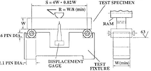
Accuracy of the ηηηη factor approach for deeply cracked sub sized SE(B) specimens
The applicability of the ASTM formula (2008) for SE(B) specimens is examined here for sub sized specimen. The values of the width W and the span S (Figure 4) are respectively of 10 and 40 mm. The specimens are not side grooved and their initial cracks exceed the half width W/2.
Figure 4: Bend test fixture design (ASTM 2008)
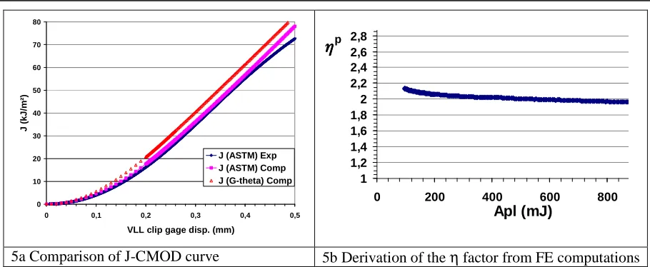
0 10 20 30 40 50 60 70 80
0 0,1 0,2 0,3 0,4 0,5
VLL clip gage disp. (mm)
J ( k J /m ²)
J (ASTM) Exp J (ASTM) Comp
J (G-theta) Comp 1
1,2 1,4 1,6 1,8 2 2,2 2,4 2,6 2,8
0 200 400 600 800
Apl (mJ)
Ü Ü Ü
Üp
5a Comparison of J-CMOD curve 5b Derivation of the η factor from FE computations
Figure 5: J and η estimations for a sub sized bend specimens
Application of the GE-EPRI estimation scheme to improve the ηηηη factor approach
The influence of the hardening exponent on the η factor has been examined by several authors (e.g. Sharobeam 1991, Ruggieri 2012). Our work aimed to have first a judgment on the accuracy of the coefficients hi (a, n) tabulated in GE-EPRI approach. The second step consisted in developing analytical
expression of these functions.
The hardening dependence of the η factor may be deduced from the GE-EPRI functions. The functions have been obtained by FE computations for a fully plastic material obeying a power law:
n σ σ α ε ε 0 0 p
= . On one hand J is given by
1 n 0 1 1 0 0 P Q Q n) (a/W; h W) (a, g ε σ α J + ⋅ ⋅ ⋅ ⋅ ⋅ = .
On the other hand the plastic work may be also expressed using the GE-EPRI functions :
n 0 3 3 0 p c p c q 0 p c Q Q n) (a/W, h W) (a, g ε α Q 1 n n = q Q 1 n n = dq Q W p c ⋅ ⋅ ⋅ ⋅ ⋅ + ⋅ + ⋅
=
∫
. In theseexpressions the functions g are given scaling lengths and the coefficients α,σ0 andε0 play no role.
We deduce that for tensile CC(T) specimen like the CC(T)
VM 3 1 p DC P k X -1 h h 1 n 1 n J J − +
= and for the
SE(B) 364 , 0 1 h h n 1 n J J 5 1 p DC P +
= . These results have been established previously by Anderson (1991).The
variations of these factors are described in the following paragraphs on the basis of our FE results.
ANALYZIS OF THE CC(T) SPECIMEN
the difference on computed η functions is small. Therefore GE-EPRI results could be used to estimate h functions although the values of h functions relative to J and LLD are inaccurate for deep cracks.
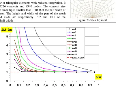
One quarter of the plate has been meshed with quadratic rectangular or triangular elements with reduced integration. It contains 3226 elements and 9940 nodes. The element size around the crack tip is smaller than 1/1000 of the half width of the specimen. The height and width of the part of the mesh represented aside are respectively 1/32 and 1/16 of the
specimen half width. Figure 7: crack tip mesh
0 1 2 3 4 5 6
0 0,1 0,2 0,3 0,4 0,5 0,6 0,7 0,8 0,9 1
a/W
J/J_Dc n=2
n=3 n=5 n=7 n=10 n=13 n=16 n=20 n=40 ETA_ASTM
Figure 6: FE computed J/JDC values as a function of crack size and hardening exponent n for the CC(T)
Figure 6 evidences a strong hardening effect on η for n < 7, but for any hardening value the results converges towards the RPP limit. The confinement condition for which the JDC formula may be used is
given by: X ≥1,372⋅n−0,384.
Asymptotic analyses and FE results, lead to the formula:
(
n 1)
X X 2 1 n2 n J
J 1,3n0,7
p DC
P
⋅ − − + − −
≈ ⋅ whose accuracy is
about 10%.
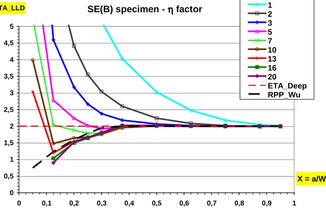
ANALYZIS OF THE SE(B) SPECIMEN
The computations have been made with the same meshes as those of the CC(T). We compared our results with those computed by C. F. Shih (1984) for checking the accuracy of the GE-EPRI solutions. An excellent agreement has been found with these results. The computations we have carried out for n = 40 are presumably less accurate. The very short crack case reveals a different behavior due to the unbounded character of the h factor at X= 0. From Shih’s asymptotic analysis (Shih, 1999) we get
X X 1 n 2 η
Lim p
LLD 0 X
− ⋅ =
→ . For the large n values, the results follow Wu’s solution obtained for a RPP
595 , 0
n 57 , 1
X ≥ ⋅ − . For all values of the hardening exponent n, the value of the relative crack size X for which the η factor RPP formulae are valid is larger for CC(T) than for SE(B) specimen, as expected.
SE(B) specimen - ηηηη factor
0 0,5 1 1,5 2 2,5 3 3,5 4 4,5 5
0 0,1 0,2 0,3 0,4 0,5 0,6 0,7 0,8 0,9 1
X = a/W
ETA_LLD 1
2 3 5 7 10 13 16 20 ETA_Deep RPP_Wu
Figure 7: FE computed η factor values as a function of crack size and hardening exponent n for the CC(T)
CONCLUSION
After recalling the bases of the η factor approach, the paper has detailed the effects of the material constitutive law and the crack depth on the variations of the η factor. In bend specimens, such as the SE(B) the stress triaxiality decreases strongly for cracks shorter than 0.3 times the specimen width. This reduces the η factor value. For tensile and bend specimens, the higher the material hardens, the higher is the η factor. Formulae have been derived to estimate critical crack sizes beyond which this loss of confinement may be neglected and that geometrical η factor may be used for toughness determination.
For the CC(T) specimen, an analytic J estimation formula has been provided. The authors are developing similar formulae for other specimens.
NOMENCLATURE
a crack depth
b remaining crack ligament
n Ramberg–Osgood strain hardening exponent Ap plastic area under the load displacement curve
B specimen thickness
E, E’ Young’s modulus under plane stress (plane strain) conditions
J J-integral
JIc critical value of J-integral
LLD Load Line Displacement
Q applied load
QL limit load
q load line displacement
qe elastic component of load line displacement qp plastic component of load line displacement SE(B) Single Edge notch Bend specimen
W structural component width α Ramberg-Osgood strain parameter
ε strain
η non-dimensional parameter describing the plastic contribution to the strain energy µ limit load factor
ν Poisson’s ratio
σ stress
σ0 Ramberg-Osgood stress parameter
REFERENCES
Anderson T. L. (1991), “Fracture Mechanics, Fundamentals and Applications”, Ed. CRC, USA, 1991. American Society for Testing and Materials (2008), Standard Test Method for Measurement of Fracture
Toughness, ASTM E1820.
Kumar V., German M. D. and Shih C. F, (1981), “An Engineering Approach for Elastic-Plastic Fracture Analysis”, rapport EPRI NP-1931, Palo-Alto, USA.
Landes J. D. and Begley, G. A. (1972), “The Effect of Specimen Geometry on JIC”, Fracture Toughness,
Proc. of the 1971 National Symposium, part II, ASTM STP 514, American Society of testing and
Materials, pp 24-39.
Landes J. D., Walter H. and Clarke, G. A. (1979), “Evaluation of Estimation Procedures used in J-Integral testing”, Elastic-Plastic Fracture, ASTM STP 668, J. D. Landes, J. A. Begley and Clarke, Eds,
American Society of testing and Materials, pp 266-287.
Rice J. R., Paris P. C. and Merkle J. G. (1973), “Some Further Results of J-Integral Analysis and Estimates”, in Progress in Flaw Growth and Fracture Toughness Testing, ASTM STP 536,
American Society for Testing and Materials, pp. 231-245.
Ruggieri C. (2012), “Further results in J and CTOD estimation procedures for SE(T) fracture specimens – Part I: Homogeneous materials”, Engineering Fracture Mechanics 79, 245–265
Shih C. F., Needleman A. (1984), “Fully Plastic Crack Problems. Part 1: Solutions by a Penalty Method. Part 2: Application of Consistency Checks”. ASME Journal of Applied Mechanics, Vol. I, 51,
March 1984, pp. 48-64”
Sumpter, J. D. G., Turner C. E. (1976) “Method for Laboratory Determination of Jc”, Cracks and Fracture ASTM STP 601, American Society for Testing and Materials, pp. 3-38.
Tada, H., Paris, P.C. and Irwin, G.R. (2000), “The Stress Analysis of Cracks Handbook”, 3rd edition, Paris Productions and Del Research Group, Missouri.
Turner C.E. (1980), “The Ubiquitous η Factor”, Fracture Mechanics 12th conference, ASTM STP 700,
1980, pp 314-337.
Sharobeam M., Landes J. D. (1991), “The load separation criterion and methodology in ductile fracture mechanics”, International Journal of Fracture, 47, 81.