ABSTRACT
HARMON, BRENDAN ALEXANDER. Tangible Landscape. (Under the direction of Eugene
Bressler and Ross Meentemeyer.)
Tangible interfaces enable users to kinaesthetically interact with computations. Theoretically
this should embody cognition in human-computer interaction so that users can cognitively grasp
digital data with their bodies and offload challenging cognitive tasks onto their bodies. I have
co-designed Tangible Landscape – a tangible interface powered by a geographic information
system – and used it to study how tangible computing mediates spatial thinking.
Tangible Landscape couples a malleable, interactive physical model of a landscape with a
digital model of the landscape so that users can 3D sketch ideas and immediately analyze
them with scientific rigor. The physical and digital models are linked through a real-time cycle of
physical interaction, 3D scanning, geospatial computation, and projection. As users interact
with a physical model of a landscape – for example by sculpting the topography – the changes
are scanned into a geographic information system (GIS), for geospatial analysis and simulation
and the resulting analytics are projected onto the physical model. My colleagues and I have
developed applications for Tangible Landscape including stormwater management, flood control,
landscape management and erosion control, trail planning, viewshed analysis, solar analysis,
wildfire management, disease spread management, invasive species management, urban
growth, and sea level rise adaption.
Tangible Landscape
by
Brendan Alexander Harmon
A dissertation submitted to the Graduate Faculty of
North Carolina State University
in partial fulfillment of the
requirements for the Degree of
Doctor of Philosophy
Design
Raleigh, North Carolina
2017
APPROVED BY:
Art Rice
Helena Mitasova
TABLE OF CONTENTS
LIST OF TABLES
. . . .
vi
LIST OF FIGURES
. . . .
vii
Chapter 1 Introduction
. . . .
1
1.1 Tangible interaction . . . .
1
1.2 Tangible geospatial interaction . . . .
1
1.2.1 Theory . . . .
2
1.2.2 Prototypes . . . .
2
1.3 Research . . . .
3
1.3.1 Methods . . . .
3
1.3.2 Results . . . .
3
1.4 Organization . . . .
4
Chapter 2 Embodied Spatial Thinking in Tangible Computing
. . . .
8
Introduction . . . .
9
Methodology . . . 10
Preliminary Results . . . 10
Future Work . . . 11
Conclusions . . . 11
Acknowledgements . . . 11
References . . . 12
Chapter 3 Tangible Landscape: Cognitively Grasping the Flow of Water
. . . .
13
Introduction . . . 14
Methods . . . 15
Results . . . 17
Discussion . . . 17
Conclusions . . . 18
References . . . 18
Chapter 4 Cognitively Grasping Topography with Tangible Landscape
. . . .
21
Introduction . . . 22
Tangible Landscape . . . 30
Coupling Experiment . . . 37
Difference Experiment . . . 51
Water Flow Experiment . . . 55
Discussion . . . 58
Future Work . . . 63
Conclusions . . . 65
Appendix A . . . 66
Appendix E . . . 72
Appendix F . . . 72
Appendix G . . . 72
References . . . 73
Chapter 5 Tangible Modeling with Open Source GIS
. . . .
78
Introduction . . . 89
System Configuration . . . 104
Building Physical 3D Models . . . 118
Basic Landscape Analysis . . . 139
Surface Water Flow and Soil Erosion Modeling . . . 151
Viewshed Analysis . . . 163
Trail Planning . . . 169
Solar Radiation Dynamics . . . 182
Wildfire Spread Simulation . . . 189
Coastal Modeling . . . 198
Appendix A . . . 203
APPENDICES
. . . .
218
Appendix A
GIS-based environmental modeling with tangible interaction and
dynamic visualization . . . 219
Introduction . . . 220
Methods . . . 221
Applications . . . 224
Discussion . . . 226
Conclusion . . . 227
Appendix B
Integrating Free and Open Source Solutions into Geospatial Science
Education . . . 228
Introduction . . . 230
Approach to Course Design and Implementation . . . 231
Course Implementation . . . 235
Future Directions . . . 238
Conclusions . . . 239
Appendix . . . 240
References . . . 242
Appendix C
Open source approach to urban growth simulation . . . 244
Introduction . . . 245
FUTURES Model . . . 246
Integration in GRASS GIS . . . 246
Case Study . . . 248
Discussion . . . 250
Conclusion . . . 250
Introduction . . . 253
System Overview . . . 253
Demonstration . . . 255
Conclusion . . . 256
References . . . 256
Table 3.1 Water depth statistics . . . 17
Table 3.2 Minimum distance statistics . . . 17
Table 3.3 Depression statistics . . . 17
Table 3.4 Depression percentages . . . 17
Table 4.1 Actuated pin table interfaces . . . 28
Table 4.2 Augmented architectural modeling interfaces . . . 28
Table 4.3 Augmented clay interfaces . . . 28
Table 4.4 Augmented sandbox interfaces . . . 29
Table 4.5 Bivariate scatterplots of elevation values . . . 43
Table 4.6 Coupling experiment: per-cell statistics and analyses . . . 45
Table 4.7 Students . . . 46
Table 4.8 Academics and professionals . . . 46
Table 4.9 Landscape architecture students . . . 47
Table 4.10 GIS students . . . 47
Table 4.11 3D novices . . . 48
Table 4.12 3D experts . . . 48
Table 4.13 Coupling experiment: percent cells . . . 49
Table 4.14 Mean minimum distance . . . 49
Table 4.15 Difference experiment . . . 53
Table 4.16 Difference experiment: per-cell statistics . . . 53
Table 4.17 Difference experiment: geospatial analyses . . . 53
Table 4.18 Difference experiment: percent cells . . . 53
Table 4.19 Difference experiment: comparison . . . 54
Table 4.20 Water flow experiment: per-cell statistics . . . 56
Table 4.21 Water flow experiment: geospatial analyses . . . 56
Table 4.22 Water flow experiment: percent cells . . . 56
Table 4.23 Water flow experiment: comparison . . . 57
Table 4.24 Interviews . . . 59
Table 4.25 How to build Tangible Landscape . . . 66
Table 5.1 Naming conventions for GRASS GIS modules . . . 112
Table 5.2 CNC settings: horizontal rough cut with MDF . . . 126
Table 5.3 CNC settings: parallel finish cut with MDF . . . 126
Table 5.4 Classes of the Anderson fuel model . . . 190
Table C.1 Predictors and estimated coefficients for the site suitability model . . . 249
LIST OF FIGURES
Figure 2.1 3D sketching with Tangible Landscape . . . 11
Figure 2.2 Standard deviation of differences . . . 11
Figure 2.3 Reference model . . . 12
Figure 2.4 Model made with projection augmented modeling . . . 12
Figure 2.5 Model made with digital sculpting . . . 12
Figure 3.1 Modeling the flow of water with Tangible Landscape . . . 15
Figure 3.2 How Tangible Landscape works . . . 15
Figure 3.3 Reference landscape with simulated water flow . . . 15
Figure 3.4 Digitally sculpting and tangibly sculpting . . . 16
Figure 3.5 Water depth anlaysis . . . 19
Figure 3.6 Depression analysis . . . 19
Figure 3.7 Difference analysis . . . 19
Figure 3.8 Detail of difference analysis . . . 19
Figure 3.9 Minimum distance for digital sculpting . . . 20
Figure 3.10 Minimum distance for tangible sculpting . . . 20
Figure 4.1 Modeling the flow of water with Tangible Landscape . . . 23
Figure 4.2 How Tangible Landscape works . . . 31
Figure 4.3 Modes of interaction with Tangible Landscape . . . 31
Figure 4.4 Scanning arms and hands as topography . . . 31
Figure 4.5 Naturally exploring subsurface soil moisture . . . 32
Figure 4.6 Collaborative 3D sketching with VR . . . 32
Figure 4.7 Software schema for Tangible Landscape . . . 34
Figure 4.8 Accuracy assessment . . . 35
Figure 4.9 Scanning accuracy . . . 35
Figure 4.10 Casting polymeric sand models with 3D printed molds . . . 36
Figure 4.11 Sculpting a terrain model using the difference analytic . . . 37
Figure 4.12 Trail planning with Tangible Landscape . . . 38
Figure 4.13 Testing coastal flood defences with Tangible Landscape . . . 38
Figure 4.14 Managing the simulated spread of termites . . . 38
Figure 4.15 Participants . . . 39
Figure 4.16 Coupling experiment: digital modeling . . . 41
Figure 4.17 Coupling experiment: analog modeling by hand . . . 41
Figure 4.18 Coupling experiment: projection augmented modeling . . . 41
Figure 4.19 Landforms identified by r.geomorphon . . . 44
Figure 4.20 Pairwise comparison by category of participants . . . 44
Figure 4.21 Water flow experiment . . . 55
Figure 4.22 Tangible Landscape with robotic fabrication . . . 65
Figure 4.23 Stickers . . . 67
Figure 5.3 inFORM . . . 94
Figure 5.4 The Tangible Geospatial Modeling System . . . 97
Figure 5.5 3D sketching a dam with Tangible Landscape . . . 98
Figure 5.6 Collaboratively sculpting a pond . . . 99
Figure 5.7 3D sketching a levee breach . . . 100
Figure 5.8 System configuration . . . 107
Figure 5.9 Mobile system setup . . . 108
Figure 5.10 Laboratory system setup . . . 109
Figure 5.11 Mesh generated by Kinect Fusion . . . 114
Figure 5.12 Calibration . . . 115
Figure 5.13 A CNC routed model of Sonoma Valley, CA . . . 119
Figure 5.14 Sculpting a polymeric sand model . . . 120
Figure 5.15 A laser cut contour model . . . 123
Figure 5.16 A CNC routed model of Jockey’s Ridge, NC . . . 124
Figure 5.17 A CNC router carving a terrain model . . . 125
Figure 5.18 How to prepare MDF for CNC routing . . . 125
Figure 5.19 Magnetic markers . . . 127
Figure 5.20 Modes of interaction using markers . . . 127
Figure 5.21 Casting polymeric sand from 3D printed molds . . . 128
Figure 5.22 Casting polymeric sand from CNC routed molds . . . 129
Figure 5.23 A thermoformed polystyrene model . . . 129
Figure 5.24 3D renderings of lidar data . . . 130
Figure 5.25 3 x 3 neighborhood around an elevation value . . . 142
Figure 5.26 Slope and aspect maps . . . 143
Figure 5.27 Profile and tangential curvature . . . 143
Figure 5.28 Landforms identified with geomorphons . . . 144
Figure 5.29 Geomorphons . . . 144
Figure 5.30 Lake Raleigh Woods . . . 145
Figure 5.31 Basic workflow with DEM differencing . . . 146
Figure 5.32 Slope and aspect of a scanned model . . . 148
Figure 5.33 Profile and tangential curvature of a scanned model . . . 148
Figure 5.34 Landform classification for a scanned model . . . 150
Figure 5.35 Flow accumulation and watershed boundaries . . . 156
Figure 5.36 Water depth computed with r.sim.water . . . 157
Figure 5.37 Erosion and deposition for a scanned model . . . 158
Figure 5.38 Lake Raleigh and it’s surroundings . . . 159
Figure 5.39 Lake Raleigh’s current conditions and a new scenario . . . 159
Figure 5.40 Flood simulation for current conditions . . . 161
Figure 5.41 Flood simulation for new scenario . . . 161
Figure 5.42 Line of sight analysis . . . 164
Figure 5.43 Lake Raleigh Woods DSM . . . 165
Figure 5.44 Placing a marker to identify a viewpoint . . . 166
Figure 5.46 Viewsheds from new buildings . . . 168
Figure 5.47 The TSP applied to a network of potential trails . . . 172
Figure 5.48 The slope and cross-slope of a trail . . . 172
Figure 5.49 Friction map for Lake Raleigh . . . 175
Figure 5.50 A trail around Lake Raleigh . . . 177
Figure 5.51 Trail analytics with Tangible Landscape . . . 179
Figure 5.52 Iteratively designing trails with Tangible Landscape . . . 180
Figure 5.53 Different configurations of buildings . . . 184
Figure 5.54 Shadows cast by different building configurations . . . 186
Figure 5.55 Direct solar irradiation . . . 187
Figure 5.56 Solar irradiation for different building configurations . . . 188
Figure 5.57 Orthophotograph and fuel map for Centennial Campus . . . 192
Figure 5.58 The simulated spread of fire without intervention . . . 194
Figure 5.59 Creating a firebreak with Tangible Landscape . . . 195
Figure 5.60 The spread of fire after creating a firebreak . . . 196
Figure 5.61 The spread of fire after creating another firebreak . . . 196
Figure 5.62 Jockey’s Ridge, Nags Head, NC . . . 199
Figure 5.63 Simulated inundation for Jockey’s Ridge . . . 200
Figure 5.64 Designs for pavilions on Roanoke Island, NC . . . 201
Figure 5.65 Siting pavilions with Tangible Landscape . . . 201
Figure 5.66 Simulated water flow and erosion for the pavilions . . . 202
Figure 5.67 Landforms in the High Tatras, Slovakia . . . 204
Figure 5.68 The evolution of Oregon Inlet . . . 204
Figure 5.69 Simulated storm surge for Rodanthe, NC . . . 205
Figure 5.70 Land change for a watershed in Charlotte, NC . . . 205
Figure 5.71 Reconstruction of a paleolake, Mongolia . . . 206
Figure 5.72 Sand models of beaches and streams . . . 207
Figure 5.73 Simulated breach of a coal ash pond . . . 208
Figure 5.74 Generating time-series data . . . 208
Figure 5.75 Interacting with disease and invasion models . . . 209
Figure 5.76 Exploring subsurface soil moisture . . . 210
Figure 5.77 Starting GRASS GIS . . . 213
Figure 5.78 Displaying raster maps . . . 213
Figure 5.79 Running GRASS GIS modules . . . 214
Figure A.1 Physical setup . . . 221
Figure A.2 Different methods of creating models . . . 222
Figure A.3 Real-time water flow modeling . . . 224
Figure A.4 The current condition of Lake Raleigh Woods . . . 225
Figure A.5 First development scenario . . . 225
Figure A.6 First modified development scenario . . . 225
Figure A.7 Second development scenario . . . 226
Figure B.3 Geospatial Modeling and Analysis assignment reports . . . 236
Figure B.4 Geospatial Modeling and Analysis exam and project paper . . . 236
Figure B.5 Students visualizing a digital elevation model . . . 237
Figure B.6 Students working on projects with Tangible Landscape . . . 238
Figure B.7 Students presenting designs for a trail system . . . 238
Figure C.1 Simplified schema of FUTURES conceptual model . . . 246
Figure C.2 Diagram of FUTURES workflow . . . 247
Figure C.3 An example of
r.future.demand
output plot . . . 247
Figure C.4 2011 land cover and protected areas in the Asheville, North Carolina . . . 248
Figure C.5 Three realizations of multiple stochastic runs with different scenarios . . . 249
Figure C.6 Area in km2 of converted land for urban sprawl and infill scenarios . . . 249
Figure D.1 Physical setup of Tangible Landscape and the proposed extension . . . 254
Figure D.2 Application process diagram . . . 254
Figure D.3 Interaction modes supported by Tangible Landscape . . . 254
Figure D.4 Sculpting topography to form ponds . . . 255
Figure D.5 Drawing patches of trees with a laser pointer . . . 256
1
Introduction
1.1 Tangible interaction
In a seminal paper Ishii and Ullmer envisioned tangible user interfaces that would ‘bridge the
gap between cyberspace and the physical environment by making digital information (bits)
tangible’ [13]. They described ‘tangible bits’ as ‘the coupling of bits with graspable physical
objects’ [13]. Tangible interfaces – interfaces that couple physical and digital data [1] – are
designed to physically manifest digital data so that users can cognitively grasp and absorb it, so
that we can think with it rather than about it [14]. Since ‘the physical state of tangibles embodies
key aspects of the digital state of an underlying computation’ [12] data is not just visualized,
but can also be felt and directly, physically manipulated, leveraging highly developed motor
skills. When interactions are embodied intention, action, and feedback should be seamlessly
connected. Interaction should be automatic, subconscious, and intuitive.
1.2 Tangible geospatial interaction
Theoretically tangible interfaces for geospatial modeling should enable intuitive digital sculpting,
streamline design processes by seamlessly integrating analog and digital workflows, and
im-prove collaboration and communication by enabling multiple users to simultaneously interact in
a natural way [21]. GIS provide the extensive libraries for geospatial databasing, processing,
analysis, modeling, simulation, and visualization needed to address real world problems [23].
Tangible interfaces for geospatial modeling have the potential to make spatial science more
intuitive by enabling a rapid iterative process of observation, hypothesizing, testing, and
infer-ence. With these systems users can for example dynamically explore how topographic form
influences landscape processes [15].
A review of tangible interfaces for geospatial modeling (Tables 4.1-4.4), however, reveals a
dearth of critical research. While many prototypes have been developed there have been few
case studies or qualitative user studies and no quantitative studies. The theories that have
inspired tangible interfaces for geospatial modeling have not yet been critiqued or proven.
1.2.2 Prototypes
1.3 Research
The aim of this research was to make scientific spatial computing natural, rapid, and collaborative
in order to streamline spatial science and design. The objective was to design a tangible interface
for geospatial modeling and study how it mediates spatial cognition in order to implement, study,
critique, and refine theories about tangibles and spatial thinking. Through an iterative cycle of
design and research my colleagues and I addressed the following research questions:
• How can we design an effective tangible interface for geospatial modeling?
• How can we use tangible geospatial analytics to solve spatial problems?
• How does coupling physical and digital models of topography mediate spatial thinking?
• How do different tangible geospatial analytics mediate spatial thinking?
• How do tangible geospatial analytics mediate how users relate form and process?
1.3.1 Methods
I co-designed Tangible Landscape and ran a series of terrain modeling experiments studying
how tangible geospatial modeling mediates spatial cognition and performance. The experiments
studied how coupling physical and digital models and providing real-time analytic feedback
affected 3D spatial performance. Spatial performance was assessed using qualitative methods
including semi-structured interviews and direct observation and quantitive methods
includ-ing geospatial modelinclud-ing, analysis, simulation, and statistics. This research has informed the
continued design and development of Tangible Landscape.
1.3.2 Results
and help users connect form to processes [5, 10].
1.4 Organization
This thesis is a collection of papers and a book about Tangible Landscape.
Chapter 2 describes a pilot study for the first terrain modeling experiment focused on coupling
digital and physical models. This chapter is a reprint of the paper
Embodied Spatial Thinking in
Tangible Computing
from the Proceedings of the TEI ’16: Tenth International Conference on
Tangible, Embedded, and Embodied Interaction [2].
Chapter 3 describes a pilot study for the third terrain modeling experiment using Tangible
Landscape’s water flow analytic. This chapter is a reprint of the paper
Tangible Landscape:
Cognitively Grasping the Flow of Water
from the International Archives of the Photogrammetry,
Remote Sensing and Spatial Information Sciences [10]
Chapter 4 describes the design of Tangible Landscape and then describes the series of terrain
modeling experiments. This chapter is a draft of the paper
Cognitively Grasping Topography
with Tangible Landscape
, which has been submitted for publication [5].
Chapter 5 describes the design of Tangible Landscape, its applications, how to set it up, and
how use it. This chapter is a reprint of the book
Tangible Modeling with Open Source GIS
[18].
Appendix A describes the first generation of Tangible Landscape and demonstrates applications.
This appendix is a reprint of the paper
GIS-based environmental modeling with tangible
interac-tion and dynamic visualizainterac-tion
published in the Proceedings of the 7th International Congress
on Environmental Modelling and Software [17].
Appendix B describes how free, open source software can be integrated into geospatial
education to promote open and reproducible science. Tangible Landscape is used in a couple
the case studies demonstrating this approach. This appendix is a reprint of the paper
Integrating
Free and Open Source Solutions into Geospatial Science Education
published in the ISPRS
Simulation) model into GRASS GIS and makes a case for GRASS GIS as a platform for free,
open source geospatial software development. This appendix is a reprint of the paper an
Open
source approach to urban growth simulation
published in The International Archives of the
Photogrammetry, Remote Sensing and Spatial Information Sciences [19].
Appendix D describes the coupling of Tangible Landscape with an immersive virtual environment
so that users can visualize and design landscapes at a human-scale. This appendix is a preprint
of the paper
Immersive Tangible Geospatial Modeling
that has been accepted for publication
in the Proceedings of the 24th ACM SIGSPATIAL International Conference on Advances in
Geographic Information Systems [22].
1. Dourish, P. Where the action is: the foundations of embodied interaction. Cambridge,
MA: MIT Press, 2001.
2. Harmon, B. A. Embodied spatial thinking in tangible computing.
Proc. TEI ’16
, 693–696.
3. Harmon, B. A. Embodied spatial thinking in tangible computing.
TEI ’16: Tangible,
Em-bedded, and Embodied Interaction 2016
. 2016.
4. Harmon, B. A. Tangible geospatial modeling for landscape architects.
2014 Geodesign
Summit
. 2014.
5. Harmon, B. A. Cognitively Grasping Topography with Tangible Landscape. Submitted for
publication. 2016.
6. Harmon, B. A. Creative spatial thinking with Tangible Landscape.
American Association
of Geographers Annual Meeting 2016
. 2016.
7. Harmon, B. A. Serious Gaming with Tangible Landscape. Raleigh, NC, 2016.
8. Harmon, B. A. Tangible geographies.
Royal Geographical Society Annual International
Conference 2016
. 2016.
9. Harmon, B. A. Tangible interaction for GIS.
FOSS4G NA 2016
. 2016.
10. Harmon, B. A. Tangible Landscape: cognitively grasping the flow of water.
The
Inter-national Archives of the Photogrammetry, Remote Sensing and Spatial Information
Sciences
. 2016.
11. Harmon, B. A. Tangible Landscape: cognitively grasping the flow of water.
International
Society of Photogrammetry and Remote Sensing 2016
. 2016.
12. Ishii, H. Tangible bits: beyond pixels.
Proc. TEI ’08
, xv–xxv.
13. Ishii, H., & Ullmer, B. Tangible bits: towards seamless interfaces between people, bits
and atoms.
Proc. CHI ’97
, 234–241.
14. Kirsh, D. Embodied cognition and the magical future of interaction design.
ACM Trans.
Comput.-Hum. Interact.
20
(1), 2013: 3:1–3:30.
15. Mitasova, H. Real-time landscape model interaction using a tangible geospatial
model-ing environment.
IEEE Computer Graphics and Applications
,
26
(4), 2006: 55–63.
16. Petras, V. Integrating Free and Open Source Solutions into Geospatial Science
Educa-tion.
ISPRS International Journal of Geo-Information
,
4
(2), 2015: 942–956.
Mod-18. Petrasova, A. Tangible Modeling with Open Source GIS. Springer, 2015.
19. Petrasova, A. Open source approach to urban growth simulation.
The International
Archives of the Photogrammetry, Remote Sensing and Spatial Information Sciences
.
2016, 953–959.
20. Piper, B. Illuminating clay: a 3-D tangible interface for landscape analysis.
Proceedings
of the SIGCHI conference on Human factors in computing systems - CHI ’02
. 2002,
355.
21. Ratti, C. Tangible User Interfaces (TUIs): A Novel Paradigm for GIS.
Transactions in
GIS
,
8
(4), 2004: 407–421.
22. Tabrizian, P. Immersive Tangible Geospatial Modeling.
Proc. SIGSPATIAL’16
.
23. Tateosian, L. TanGeoMS: tangible geospatial modeling system.
IEEE transactions on
visualization and computer graphics
,
16
(6), 2010: 1605–12.
Reprint
Brendan A. Harmon
. 2016. Embodied Spatial Thinking in Tangible Computing. In
TEI ’16:
Proceedings of the Tenth International Conference on Tangible, Embedded, and Embodied
Interaction
. Eindhoven, Netherlands: ACM Press, 693–696. DOI:
http://dx.doi.org/10.1145/
2839462.2854103
Attribution
Embodied Spatial Thinking in Tangible Computing
Brendan Alexander Harmon North Carolina State University
Raleigh, USA [email protected]
ABSTRACT
Tangible user interfaces are based on the premise that embod-ied cognition in computing can enhance cognitive processes. However, the ways in which embodied cognition in computing transform spatial thinking have not yet been rigorously studied. I have co-designed Tangible Landscape – a continuous shape display powered by a geographic information system – and used it to explore how technology mediates spatial cognition in a rigorous experiment.
In this terrain modeling experiment I use geospatial analytics to analyze how visual computing with a GUI and tangible computing with a shape display mediate multidimensional spatial performance.
My initial findings suggest that:1.digital sculpting via a GUI is unintuitive,2.shape displays like Tangible Landscape can be intuitive, enhance spatial performance, and enable rapid iteration and ideation, and3.different analytics encourage significantly different modes of spatial thinking and strategies for modeling.
ACM Classification Keywords
H.5.2. Information Interfaces and Presentation (e.g. HCI): User Interfaces – Evaluation/methodology; Interaction styles; Prototyping; Theory and methods
Author Keywords
Human-computer interaction; tangible user interfaces; tangible interaction; embodied cognition; spatial thinking; 3D modeling
INTRODUCTION
In embodied cognition the mind is embedded in the body. Higher cognitive processes rely on lower level processes such as emotion and sensorimotor processes that link perception and action [2]. Thus body and action mediate thought. Cognitive processes can be physically simulated with cognition offloaded onto action. Objects such as tools can be cognitively grasped and temporarily, contingently incorporated into ones body
Permission to make digital or hard copies of all or part of this work for personal or classroom use is granted without fee provided that copies are not made or distributed for profit or commercial advantage and that copies bear this notice and the full citation on the first page. Copyrights for components of this work owned by others than ACM must be honored. Abstracting with credit is permitted. To copy otherwise, or republish, to post on servers or to redistribute to lists, requires prior specific permission and/or a fee. Request permissions from [email protected].
TEI ’16, February 14-17, 2016, Eindhoven, Netherlands. Copyright © 2016 ACM ISBN/978-1-4503-3582-9/16/02$15.00. DOI http://dx.doi.org/10.1145/2839462.2854103
schema [5]. This view of cognition considers feeling, action, and perception to be functionally integral to thought. Based on the theory of embodied cognition researchers have theorized a physical-digital divide in human-computer inter-action – positing that the high level of abstrinter-action required to interact with a computer via a graphical user interface (GUI) in a visual computing paradigm constrains how we think – and designed innovative technologies for bridging this divide such as tangible user interfaces (TUIs) [3, 1]. TUIs are de-signed to physically manifest digital data as tangible bits that afford the ability to directly, physically feel and manipulate data [3]. TUIs make pragmatic representations of digital data. Pragmatic representations are conceptual models for rapidly generating action that are primarily based on tactile feedback and are processed automatically, immediately, and subcon-sciously [4]. By physically manifesting data so that we can pragmatically interact with computations, TUIs should enable rapid, intuitive action and expression in a way that was not possible in visual computing. By enabling embodied cognition in human-computer interaction TUIs should let us cognitively grip data as an extension of our bodies, intuitively manipulate data, and physically simulate processes. This should enhance spatial thinking.
Research on TUIs has been more focused on the design and development of the technology than empirically testing the use and effects of the technology. Rasmussen et al. for example discuss the focus on the design and development of shape displays rather than empirical research about their use. [7]. Research on tangible interaction has focused on user experi-ence and to a lesser degree user performance using methods such as participant observation, semi-structured interviews, video analysis, and small-scale experiments.
While the theory of embodied cognition has inspired the design of novel technologies for human-computer interaction, its applied principles need to be empirically tested, critiqued, and refined in order to improve interaction design. The aim of this research is to study how tangible computing mediates spatial thinking in order to improve interaction design, enhance spatial performance, and improve spatial education.
Testable hypotheses I hypothesize that:
1. limited feedback constrains spatial performance, 2. misinterpretations of 3D space in visual computing reduce
3. computational analytics like differencing and flow simula-tions can enhance spatial performance,
4. computationally enriched analytical thinking can be coordi-nated with embodied thinking,
5. tangible computing that computationally enhances embod-ied spatial thinking can improve spatial performance, and 6. tangible computing can enable a rapid iterative process
of exploratory, generative form-finding that can improve spatial performance.
METHDOLOGY
I have conducted a rigorous experiment using geospatial ana-lytics to compare spatial performance in analog modeling by hand, in tangible computing using Tangible Landscape, and in visual computing using 3D modeling programs via a GUI. Tangible Landscape is a continuous shape display tightly inte-grated with GRASS GIS that was designed to intuitively 3D sketch landscapes (Figure 1). Conceptually, Tangible Land-scape couples a physical model with a digital model in a real-time feedback cycle of 3D scanning, geospatial modeling and simulation, and projection (Figure 1a) [6].
I have begun to test my hypotheses using quantitative meth-ods Rather than studying basic spatial cognitive abilities that can not usefully be disentangled in applied use, I am study-ing applied spatial cognitive processes usstudy-ing the metrics and parameters of the given application. I am studying how partic-ipants perform in a series of time constrained terrain modeling exercises using analog modeling, visual computing, and tan-gible computing. 6 landscape architects and 6 geospatial ana-lysts have participated in this pilot study. I am assessing their performance with each technology using spatial statistics, to-pographic parameters, morphology, process-form interactions, and differencing.
Terrain modeling experiment
The 1stexercise tests spatial performance in analog modeling to establish the baseline spatial ability of each participant. In this exercise participants sculpt a given terrain in polymeric sand using their hands with a CNC routed model for reference. The 2ndexercise tests spatial performance in projection aug-mented analog modeling to establish a baseline for spatial performance in tangible computing. In this exercise partici-pants sculpt a given terrain in polymeric sand using a projected map of the given elevation and contours as a guide. The 3rd-5thexercises test spatial performance in tangible com-puting augmented with different analytics. In the 3rdexercise participants use Tangible Landscape to sculpt a given terrain in polymeric sand using the given and scanned contours as a guide. In the 4thexercise participants use Tangible Landscape to sculpt a given terrain in polymeric sand using the difference between the given and the scanned landscape as a guide. In the 5thexercise participants use Tangible Landscape to sculpt a given terrain in polymeric sand using the simulated water flow over the scanned landscape as a guide in order to study 4D thinking.
The 6thand 7thexercises test spatial performance in visual computing. In the 6thexercise participants digitally sculpt a given terrain in Rhinoceros, a 3D modeling program, using the given 3D contours as a guide. In the 7thexercise participants digitally sculpt a given terrain in VUE, a 3D modeling program designed for intuitive terrain sculpting, with a CNC routed model for reference.
Data collection and analysis
In the 1st-5thexercises the resulting physical models are 3D scanned, imported into GRASS GIS as point clouds, and inter-polated as DEMs for analysis. In the 6thand 7thexercises the resulting digital models are exported as point clouds, imported into GRASS GIS, and interpolated as DEMs for analysis. For each model I compute the elevation and its histogram and bi-variate scatterplot, the slope, the difference and its histogram, the simulated water flow, and morphology. For each exercise I compute a map of the coefficient of variance of all the of DEMs, bivariate scatterplots of the covariance and correlation matrix of all the of DEMs, and the mean and the absolute value of the mean of the differences between the the reference terrain and the modeled terrain.
Code
As a work of open science the data and the python scripts for data analysis are publicly available on GitHub athttps: //github.com/baharmon/tangible_topographyreleased under the GNU General Public License version 2. Both GRASS GIS and Tangible Landscape are open source projects released under the GNU General Public License version 2. Tangi-ble Landscape is availaTangi-ble on GitHub athttps://github.com/ ncsu-osgeorel/grass-tangible-landscape.
PRELIMINARY RESULTS
Select results for one participant in the pilot study are shown in Figures 3, 4, and 5.
(a) (b) (c) (d)
Figure 1. 3D sketching with Tangible Landscape: (a) a cycle of scanning and projection couples a physical and digital model, (b) the differencing analytic with blue where sand should be added and red where sand should be removed, (c) a participant adding sand, and (d) the updated differencing analytic.
ones ability to critique the model and refine its form,2.shape displays like Tangible Landscape can be intuitive, enhance spatial performance, and enable rapid iteration and thus cre-ative spatial learning.3.digital sculpting via a graphical user interface is unintuitive and visually ambiguous leading to mis-interpretations of depth, height, and interior space.
(a) (b)
Figure 2. Standard deviations of the differences for all partici-pants: (a) in Ex. 2 using projection augmented modeling and (b) in Ex. 6 using Rhinoceros.
FUTURE WORK
The full study will have approximately 40 participants. Based on the results of the study I hope to develop a theory of how technology mediates spatial cognition. In the long-term I plan to expand this study of embodied spatial cognition in tangible computing as a collaborative research project with psychologists using spatial analytics, eye tracking, biometric sensors, and EEGs.
CONCLUSIONS
This study is unique in applying geospatial analyses to asses spatial performance in tangible interaction. My initial find-ings suggest that shape displays like Tangible Landscape can with the right computational analytics enhance performance in novel ways and enable rapid iterations of generative form-finding and critical analysis. Different analytics encourage significantly different modes of spatial thinking and strategies for modeling. The differencing analytic leads to significant improvements in spatial performance and enables an iterative process.
ACKNOWLEDGMENTS
My colleagues in the NCSU Open Source Geospatial Research and Education Lab (http://geospatial.ncsu.edu/osgeorel/)
Anna Petrasova, Vaclav Petras, Helena Mitasova, and Ross Meentemeyer contributed to this research by collaboratively designing Tangible Landscape and helping to run the experi-ment.
REFERENCES
1. Paul Dourish. 2001.Where the action is: the foundations of embodied interaction. MIT Press, Cambridge, MA. 2. Benoit Hardy-Vallée and Nicolas Payette. 2008.Beyond
the Brain: Embodied, Situated and Distributed Cognition. Cambridge Scholars Publishing, Newcastle, UK. 3. Hiroshi Ishii and Brygg Ullmer. 1997. Tangible bits:
towards seamless interfaces between people, bits and atoms. InProceedings of the SIGCHI conference on Human factors in computing systems - CHI ’97. ACM Press, 234–241.DOI:
http://dx.doi.org/10.1145/258549.258715
4. Marc Jeannerod. 1997.The Cognitive Neuroscience of Action. Blackwell, Cambridge, MA. 236 pages. 5. David Kirsh. 2013. Embodied cognition and the magical
future of interaction design.ACM Transactions on Computer-Human Interaction20, 1 (2013), 3:1–3:30.
DOI:http://dx.doi.org/10.1145/2442106.2442109
6. Anna Petrasova, Brendan Harmon, Vaclav Petras, and Helena Mitasova. 2015.Tangible Modeling with Open Source GIS. Springer.
7. Majken K Rasmussen, Esben W Pedersen, Marianne G Petersen, and Kasper Hornbaek. 2012. Shape-Changing Interfaces : A Review of the Design Space and Open Research Questions.Proceedings of the 2012 ACM annual conference on Human Factors in Computing Systems CHI 12(2012), 735–744.DOI:
(a)
(b)
(c)
Figure 3.Reference model: (a) the digital elevation model (DEM), (b) the difference between the refer-ence DEM and the referrefer-ence DEM, and (c) the bivariate scatterplot of the dif-ference between the redif-ference DEM and the reference DEM.
(a)
(b)
(c)
Figure 4. Participant’s model for Ex. 2 using projection augmented modeling:
(a) the DEM,
(b) the difference between the partic-ipant’s DEM and the reference DEM, and
(c) the bivariate scatterplot of the dif-ference between the participant’s DEM and the reference DEM.
(a)
(b)
(c)
Figure 5. Participant’s model for Ex. 6 using digital sculpting with Rhinoceros:
(a) the DEM,
3
Tangible Landscape: Cognitively Grasping the Flow of Water
Reprint
Brendan A. Harmon
, Anna Petrasova, Vaclav Petras, Helena Mitasova, and Ross K.
Meente-meyer. 2016. Tangible Landscape: cognitively grasping the flow of water. In
The International
Archives of the Photogrammetry, Remote Sensing and Spatial Information Sciences
. Prague:
International Society of Photogrammetry and Remote Sensing. DOI:
http://dx.doi.org/10.
5194/isprsarchives-XLI-B2-647-2016647
Attribution
TANGIBLE LANDSCAPE: COGNITIVELY GRASPING THE FLOW OF WATER
B. A. Harmona⇤, A. Petrasovaa, V. Petrasa, H. Mitasovaa, R. K. Meentemeyera
aCenter for Geospatial Analytics, North Carolina State University - (baharmon, akratoc, vpetras, hmitaso, rkmeente)@ncsu.edu
KEY WORDS:embodied cognition, spatial thinking, physical processes, water flow, hydrology, tangible user interfaces, user experi-ment, 3D
ABSTRACT:
Complex spatial forms like topography can be challenging to understand, much less intentionally shape, given the heavy cognitive load of visualizing and manipulating 3D form. Spatiotemporal processes like the flow of water over a landscape are even more challenging to understand and intentionally direct as they are dependent upon their context and require the simulation of forces like gravity and momentum. This cognitive work can be offloaded onto computers through 3D geospatial modeling, analysis, and simulation. Inter-acting with computers, however, can also be challenging, often requiring training and highly abstract thinking. Tangible computing – an emerging paradigm of human-computer interaction in which data is physically manifested so that users can feel it and directly manipulate it – aims to offload this added cognitive work onto the body. We have designed Tangible Landscape, a tangible interface powered by an open source geographic information system (GRASS GIS), so that users can naturally shape topography and interact with simulated processes with their hands in order to make observations, generate and test hypotheses, and make inferences about scientific phenomena in a rapid, iterative process. Conceptually Tangible Landscape couples a malleable physical model with a digital model of a landscape through a continuous cycle of 3D scanning, geospatial modeling, and projection. We ran a flow modeling exper-iment to test whether tangible interfaces like this can effectively enhance spatial performance by offloading cognitive processes onto computers and our bodies. We used hydrological simulations and statistics to quantitatively assess spatial performance. We found that Tangible Landscape enhanced 3D spatial performance and helped users understand water flow.
INTRODUCTION
Understanding physical processes
Physical processes like the flow and dispersion of water are chal-lenging to understand because they unfold in time and space, are controlled by their context, and are driven by forces like gravity and momentum. The flow of water across a landscape is con-trolled by the morphological shape and gradient of the topogra-phy. It is challenging to understand how water will flow across a landscape because one must not only understand how the shape and gradient of the terrain control the flow and dispersion of water locally, but also how water will flow between shapes and gradi-ents – how the morphology is topologically connected. Under-standing a physical process requires thinking at and across multi-ple spatial scales simultaneously.
This cognitive work can be offloaded onto computers through 3D geospatial modeling, analysis, and simulation. Interacting with computers, however, can also be challenging, requiring training and highly abstract thinking that adds a new cognitive burden.
Tangible interfaces for GIS
Tangible interfaces are designed to make interaction with com-puters easier and more natural by physically manifesting digital data so that users can cognitively grasp it as an extension of their bodies, offloading cognition onto their bodies. In embodied cog-nition higher cognitive processes are built upon and grounded in sensorimotor processes – upon bodily action, perception, and ex-perience – so thinking can be performed subconsciously through action and extended with tools (Kirsh, 2013). Tangible interfaces have been developed for geographic information systems (GIS) to ease the cognitive burden of complex spatial reasoning, spatial vi-sualization, and human-computer interaction by embodying these
⇤Corresponding author
processes. Theoretically tangible interfaces for GIS should help users understand environmental processes by giving multidimen-sional geospatial data an interactive, physical form that they can cognitively grasp and kinaesthetically explore in space and time.
In a seminal paper Ishii and Ullmer envisioned tangible user in-terfaces that would ‘bridge the gap between cyberspace and the physical environment by making digital information (bits) tangi-ble’ (Ishii and Ullmer, 1997). They described ‘tangible bits’ as ‘the coupling of bits with graspable physical objects’ (Ishii and Ullmer, 1997). Tangible interfaces like Urp (Underkoffler and Ishii, 1999), Illuminating Clay (Piper et al., 2002a), and Sand-Scape (Ratti et al., 2004) enriched physical models of urban spaces and landscapes with spatial analyses and simulations like wind direction, cast shadow, slope, aspect, curvature, and water direc-tion in order to enhance and streamline spatial thinking, design, and decision-making.
Many of the analyses used in Illuminating Clay were adapted from the open source GRASS GIS project (Piper et al., 2002b) and eventually Illuminating Clay was coupled with GRASS GIS to draw on its extensive libraries for spatial computation. The aim of coupling Illuminating Clay with GRASS GIS was to ‘explore relationships that occur between different terrains, the physical parameters of terrains, and the landscape processes that occur in these terrains’ (Mitasova et al., 2006). The effort to couple a physical landscape model with GRASS GIS led to the develop-ment of the Tangible Geospatial Modeling System (Tateosian et al., 2010) and Tangible Landscape (Fig. 1) (Petrasova et al., 2014, Petrasova et al., 2015).
Figure 1: Tangibly modeling the flow of water with Tangible Landscape
that users can easily sculpt forms in a medium that will hold its shape, has good plasticity, and has a familiar feel and aesthetic. As users sculpt the physical model the model is 3D scanned and interpolated in GIS as a digital elevation model. The digital el-evation model is used to compute geospatial analyses, models, and simulations, which are then projected back onto the physical model – all in near real-time. Conceptually, this enables users to hold a GIS in their hands – feeling the shape of the earth, sculpting its topography, and directing the flow of water. This should enable users to naturally model topography and interact with simulated physical processes in a rapid, iterative process of observation, hypothesis generation and testing, and inference.
GRASS GIS geospatial computation 3D scanning projection interaction point cloud processing
Figure 2: How Tangible Landscape works: a near real-time feedback cycle of interaction, 3D scanning, point cloud
processing, geospatial computation, and projection
Cognitively grasping spatial processes
The aim of this research was to study how tangible interfaces for GIS mediate spatial thinking about landscape processes like water flow. Theoretically a tangible interface for a GIS that en-ables intuitive digital sculpting while providing analytical feed-back should allow users to dynamically explore how topographic form influences landscape processes. With a physical model one can cognitively grasp topographic form, offloading the cognitive work of understanding and shaping topographic form onto the body. A GIS can offload the cognitive work of simulating com-plex physical processes like the flow of water through computa-tion. With these physical and computational affordances com-bined in a tangible interface for GIS users should be able to more easily understand and shape spatial processes. We empirically tested how a tangible interface for GIS mediated spatial perfor-mance in a water flow modeling experiment.
METHODS
We conducted a terrain and water flow modeling experiment in which participants tried to recreate a given landscape. We quan-titatively assessed their spatial performance using hydrological simulation, summary statistics, and cell-by-cell statistics.
Flow modeling experiment
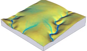
In the experiment 11 participants were asked to sculpt a given landscape using different technologies – first using Vue, a trian-gulated irregular network based 3D modeling program designed for intuitive terrain sculpting, and then using Tangible Landscape. The participants were asked to model a real landscape – a region of Lake Raleigh Woods in Raleigh, North Carolina – using each technology. We selected a region of the landscape with distinc-tive, clearly defined landforms – a central ridge flanked by two stream valleys (see Fig. 3). The digital elevation model (DEM) for this region was derived from a 2013 airborne lidar survey us-ing the regularized spline with tension interpolation method.
In the 1stexercise each participant had 10 minutes to digitally
sculpt the topography of the study landscape in Vue’s terrain ed-itor using a physical model as a reference (see Fig. 4a). Partic-ipants were given a 2 minute introduction to terrain sculpting in Vue and then 10 minutes to experiment and become familiar with the interface before beginning the exercise. Vue’s terrain edi-tor was designed to emulate sculpting by hand – there are tool brushes that are analogous to basic actions in sculpture including pushing, pulling, and smoothing.
In the 2ndexercise each participant had ten minutes to sculpt the
study landscape in polymer enriched sand using Tangible Land-scape’s water flow simulation as a guide (see Fig. 4b). As par-ticipants sculpted they could switch between projected maps of either thea)simulated water flow across the given landscape that they were trying to replicateb)or the simulated water flow across the scanned landscape.
(a) (b)
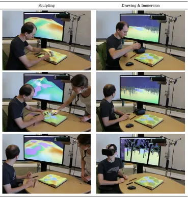
Figure 4: (a) Digitally sculpting with Vue in the 1stexercise and (b) tangibly sculpting with Tangible Landscape in the 2ndexercise
Implementation
We used GRASS GIS both for geospatial computation with Tan-gible Landscape and for the analysis of the results of the exper-iment. The algorithms used in GRASS GIS are based on peer-reviewed scientific publications and have been transparently im-plemented with free, publicly available, version controlled source code. Open, transparent algorithms are needed to fully reproduce computational science (Rocchini and Neteler, 2012). In this ex-periment we used the overland flow hydrologic simulation using a path sampling method (SIMWE) implemented in GRASS GIS as the module r.sim.water.
Shallow overland flow We simulated shallow overland water flow controlled by spatially variable topography, soil, landcover, and rainfall parameters using the SIMWE model to solve the con-tinuity and momentum equations for steady state water flow with a path sampling method. Shallow water flow can be approxi-mated by the bivariate form of the St Venant equation:
@h(r, t)
@t =ie(r, t) r ·q(r, t) (1)
where:
r(x, y)is the position [m]
tis the time [s]
h(r, t)is the depth of overland flow [m]
ie(r, t)is the rainfall excess [m/s]
(rainfall infiltration vegetation intercept)
q(r, t)is the water flow per unit width [m2
/s]. By integrating a diffusion term/ r2
[h5/3
(r)]into the solution of the continuity and momentum equations for steady state water flow diffusive wave effects can be approximated so that water can flow through depressions.
"(r)
2 r
2
[h5/3
(r)] +r ·[h(r)v(r)] =ie(r) (2)
where:
"(r)is a spatially variable diffusion coefficient.
This equation is solved using a Green’s function Monte Carlo path sampling method (Mitasova et al., 2004).
Data collection and analysis
We used summary and cell-by-cell statistics to compare the re-sults of each exercise using the reference landscape as a base-line. The digital models sculpted in the 1stexercise were
manu-ally georeferenced and imported into GRASS GIS as point clouds for modeling and analysis. The final state of the physical models sculpted in 2ndexercise were automatically 3D scanned,
georef-erenced, and imported into GRASS GIS as points clouds with Tangible Landscape for modeling and analysis. All of the point clouds were randomly resampled and interpolated as DEMs us-ing the regularized spline with tension interpolation method (Mi-tasova et al., 2005). For each model we simulated shallow over-land water flow, identified depressions, and computed the differ-ence between the modeled and referdiffer-ence water flow depth. To compute the difference we subtracted the modeled values from the initial, reference values. We identified and computed the depth of depressions by generating a depressionless DEM and then calculating the difference between the DEM from the de-pressionless DEM. Then we computed the mean, sum, and max-imum of the water depths, the depressions, and the difference in water depths for each exercise in the experiment. We visually as-sessed the spatial pattern of water flow and continuity using these maps. In order to quantitatively compare how well the modeled streams matched the reference stream we computed the distance between cells with concentrated water flow in the reference depth map and mean of the modeled depth maps. First we extracted points for each cell with high water depth values (>= 0.05ft) in the reference water depth raster and the mean water depth raster for each exercise. Then we calculated the minimum distance be-tween the reference points and the nearest points from each ex-ercise. In order to quantitatively compare the continuity of flow we computed the percentage of cells with depressions for each exercise.
Code and data
GRASS GIS is available athttps://grass.osgeo.org/ un-der the GNU GPL. Tangible Landscape is available athttps:// github.com/ncsu-osgeorel/grass-tangible-landscape
under the GNU GPL. To build your own Tangible Landscape see the documentation in the GitHub repository and refer to the book Tangible Modeling with Open Source GIS (Petrasova et al., 2015).
While the rest of the software used in this research is free and open source, Vue1is proprietary software. We used Vue’s terrain
editor for this study because it was designed specifically for in-tuitive terrain modeling, but open source 3D modeling programs like Blender2could be substituted for Vue.
RESULTS
The models sculpted with Tangible Landscape more accurately replicated the flow of water over the study landscape. The digi-tally sculpted models tended to have more diffuse water flow and more water pooling in depressions, whereas the tangibly sculpted models tended to have more concentrated flow in stream channels and less pooling in depressions. Furthermore, the spatial distribu-tion of water flow on the tangibly sculpted models more closely fit the distribution of water flow on the reference landscape.
Exercise Mean Max Sum Reference 0.01 0.47 786.25
Digital 0.21 1.83 3.60 Tangible 0.27 2.31 4.60
Table 1: Highest mean, maximum, and summed water depths (ft)
Exercise Mean Sum Digital 21.13 29244 Tangible 18.59 25724
Table 2: The minimum distances from reference stream cells to the nearest modeled cell with concentrated flow (ft)
Exercise Max Sum Reference 0.10 0.62 Digital 24.5 53 Tangible 22.2 44
Table 3: Highest max and summed depth of depressions (ft) Exercise Cells
Reference 0% Digital 44% Tangible 17.66%
Table 4: Percent of cells with depressions (3 ft2)
The models sculpted with Tangible Landscape had more concen-trated flow in stream channels with higher mean, maximum, and summed water depths (see Table 1). Fig. 6 shows that water flow in the 2ndexercise was spatially concentrated in the upper stream
channel, the lower stream channel, and the nascent swale to the right.
Furthermore the water flow across models sculpted with Tangible Landscape more closely fit the reference. Fig. 8 and the details in
1http://www.e-onsoftware.com/products/vue/ 2https://www.blender.org/
Fig. 9 show that water flow in the 1stexercise was more spatially
diffuse and dispersed, whereas water flow in the 2ndexercise was
a better fit. Fig. 10 - 11 show how well the flow of the digitally and tangibly sculpted models fit the reference flow. The digi-tally sculpted models tended to loosely fit the upper stream with fewer, more dispersed clusters of concentrated flow at further dis-tances from the reference on average. They also tended to have very few clusters at considerable distance from the swale on the right and small, dispersed clusters that tightly fit the lower stream. The tangibly sculpted models, however, tended to more densely, tightly fit the upper stream and the swale on the right. The tangi-bly sculpted models tended to miss or misplace the lower stream channel (siting it too far southeast). The near-real time water flow analytic was not very useful for modeling the lower stream segment because there was not enough contributing area on the model to generate much concentrated flow. Water flow over the sculpted models was only computed over the model, whereas the reference water flow was computed over the entire watershed. Overall the tangibly sculpted models fit the reference flow 8.32% better than the digitally sculpted models (see Table 2). The digitally sculpted models had higher max and summed water depth in depressions (see Table 1). Furthermore the depressions covered 26.34% more area of the digitally sculpted models than the tangibly sculpted models (see Table 4, Fig. 5, and Fig. 7). The presence of large depressions on the central ridge in the 1st
exer-cise reveals concave topographic morphology where there should be convex morphology. The pervasive presence of depressions in the stream channels in both exercises reveals disrupted flows with broken continuity where water should be flowing.
DISCUSSION
The modeling results show that participants tended not to clearly understand how topography directs water flow, but began to learn about the importance of curvature and continuity with the aid of the tangible interface.
When digitally sculpting participants typically focused on mak-ing the streams lower than the surroundmak-ing topography, but not on draining water into the streams or directing a continuous flow downstream. In the 1stexercise participants made low points
ap-proximately where the streams should be, but tended not to grade smooth slopes with appropriate curvature. The participants use of concave rather than convex morphology on the central ridge reveals that some did not understand how topographic curvature controls water flow. The extensive depressions distributed widely across the terrain demonstrate that participants tended not under-stand the importance of topographic curvature and continuity for water flow.
With the tangible interface they typically focused on directing water into streams, but did not tend focus on directing a contin-uous flow downstream. In the 2ndexercise participants tended
to grade smoother slopes with fewer depressions whose curva-ture directed water towards channels, concentrating it in streams. They, however, did not tend to grade the channels to continu-ously slope downstream. While participants performance im-proved substantially in the 2ndexercise, the pervasive presence
of depressions in the stream channels in both exercises demon-strates that participants did not fully understand the morphology of streams by the end of the experiment.
performance in the 2ndexercise shows that they successfully
inte-grated the tangible interface’s water flow analytic into their mod-eling process. To improve their performance they must have been able to successfully manage the added cognitive load of the an-alytical feedback. The tangibility of the interface may have let them offload some of the cognitive work of sensing and shaping 3D form onto their bodies so that they could focus on water flow. While their performance did improve in the 2ndexercise, it may
still have been adversely affected by emotions like frustration. If the cognitive load of simultaneously modeling 3D form and wa-ter flow became too great – if participants were unable to fluidly connect cause (topographic form) and effect (flow) – they might become frustrated and demotivated. Future research should in-vestigate the role of affect, motivation, and metacognition in tan-gible interaction.
More analytics may enhance participants’ understanding of wa-ter flow and stream morphology. Identifying and computing the depth of depressions highlighted the role of topographic curva-ture and continuity in water flow. While topographic parameters such as curvature and slope would highlight important aspects of the morphology, an additional step of reasoning and imagination is required to link these parameters to water flow. The ponding of water in depressions directly links topographic controls and wa-ter flow and thus should be a more intuitive analytic. We propose combining shallow overland water flow with ponding in depres-sions as an analytic to help users understand how water flows.
CONCLUSION
Tangible Landscape’s water flow analytic enabled an iterative cy-cle of form-finding and critical assessment that helped partici-pants learn how form controls process. Seeing the water flow simulation update in near real-time enabled participants to gen-erate hypotheses, test hypotheses, and draw inferences about the way that water flows over topography. As one participant said, ‘seeing the flow takes away the mystery of topography.’ Phys-ically manifesting topographic data enables users to cognitively grasp the terrain. Coupling tangible topography with the simu-lated flow of water lets users understand the simulation with their body.
REFERENCES
Ishii, H. and Ullmer, B., 1997. Tangible bits: towards seamless interfaces between people, bits and atoms. In: Proceedings of the SIGCHI conference on Human factors in computing systems - CHI ’97, ACM Press, New York, New York, USA, pp. 234–241. Kirsh, D., 2013. Embodied cognition and the magical future of interaction design. ACM Transactions on Computer-Human In-teraction20(1), pp. 3:1–3:30.
Mitasova, H., Mitas, L. and Harmon, R., 2005. Simultaneous spline approximation and topographic analysis for lidar elevation data in open-source GIS.IEEE Geoscience and Remote Sensing Letters2, pp. 375–379.
Mitasova, H., Mitas, L., Ratti, C., Ishii, H., Alonso, J. and Har-mon, R. S., 2006. Real-time landscape model interaction using a tangible geospatial modeling environment. IEEE Computer Graphics and Applications26(4), pp. 55–63.
Mitasova, H., Thaxton, C., Hofierka, J., McLaughlin, R., Moore, A. and Mitas, L., 2004. Path sampling method for modeling over-land water flow, sediment transport, and short term terrain evolu-tion in Open Source GIS. Developments in Water Science55, pp. 1479–1490.
Petrasova, A., Harmon, B. A., Petras, V. and Mitasova, H., 2014. GIS-based environmental modeling with tangible interaction and dynamic visualization. In: D. Ames and N. Quinn (eds), Proceed-ings of the 7th International Congress on Environmental Mod-elling and Software, International Environmental ModMod-elling and Software Society, San Diego, California, USA.
Petrasova, A., Harmon, B., Petras, V. and Mitasova, H., 2015.
Tangible Modeling with Open Source GIS. Springer.
Piper, B., Ratti, C. and Ishii, H., 2002a. Illuminating clay: a 3-D tangible interface for landscape analysis. In:Proceedings of the SIGCHI conference on Human factors in computing systems - CHI ’02, ACM Press, Minneapolis, p. 355.
Piper, B., Ratti, C. and Ishii, H., 2002b. Illuminating Clay: A Tangible Interface with potential GRASS applications. In: Pro-ceedings of the Open Source GIS - GRASS users conference 2002, Trento, Italy.
Ratti, C., Wang, Y., Ishii, H., Piper, B., Frenchman, D., Wilson, J. P., Fotheringham, A. S. and Hunter, G. J., 2004. Tangible User Interfaces (TUIs): A Novel Paradigm for GIS. Transactions in GIS8(4), pp. 407–421.
Rocchini, D. and Neteler, M., 2012. Let the four freedoms paradigm apply to ecology. Trends in Ecology and Evolution
27(6), pp. 310–311.
Tateosian, L., Mitasova, H., Harmon, B. A., Fogleman, B., Weaver, K. and Harmon, R. S., 2010. TanGeoMS: tangible geospatial modeling system.IEEE transactions on visualization and computer graphics16(6), pp. 1605–12.
(a) (b) (c)
Figure 5: (a) The depth of simulated water flow across the reference landscape, (b) the mean depth using digital modeling, (c) and the mean depth using tangible modeling
(a) (b) (c)
Figure 6: (a) The depth of depressions in the reference landscape, (b) the maximum depth of depressions using digital modeling, (c) and the maximum depth of depressions using tangible modeling
(a) (b) (c)
Figure 7: (a) The difference of the reference landscape, (b) the mean of digitally sculpted models, (c) and the mean of tangibly sculpted modelsfrom the reference landscape
(a) (b)
Figure 8: Detail of the difference of (a) the mean of digitally sculpted models and (b) the mean of tangibly sculpted modelsfrom the reference landscape
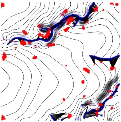
Figure 9: The lines represent the minimum distance between blue points with high concentrated flow from the reference and red points with high concentrated flow from the mean depth of digitally sculpted models