How to explain and predict the shape parameter of the generalized extreme
value distribution of streamflow extremes using a big dataset
Hristos Tyralis1, Georgia Papacharalampous2, and Sarintip Tantanee3
1Air Force Support Command, Hellenic Air Force, Elefsina Air Base, 192 00 Elefsina, Greece (https://orcid.org/0000-0002-8932-4997)
2Department of Water Resources and Environmental Engineering, School of Civil Engineering, National Technical University of Athens, Iroon Polytechniou 5, 157 80 Zografou, Greece (https://orcid.org/0000-0001-5446-954X)
3Department of Civil Engineering, Engineering Faculty, Naresuan University,
Nakhonsawan – Phitsanulok Rd., 650 00 Phitsanulok, Thailand
Corresponding author: Hristos Tyralis ([email protected])
This is a pre-print of an article published in Journal of Hydrology (2019). The final
authenticated version is available online at:
https://doi.org/10.1016/j.jhydrol.2019.04.070.
Please cite this article as:
Tyralis H, Papacharalampous G, Tantanee S (2019) How to explain and predict the shape parameter of the generalized extreme value distribution of streamflow extremes using a big dataset. Journal of Hydrology 574:628–645. doi:10.1016/j.jhydrol.2019.04.070
Abstract: The finding of important explanatory variables for the location parameter and the scale parameter of the generalized extreme value (GEV) distribution, when the latter is used for the modelling of annual streamflow maxima, is known to have reduced the uncertainties in inferences, as estimated through regional flood frequency analysis frameworks. However, important explanatory variables have not been found for the GEV shape parameter, despite its critical significance, which stems from the fact that it determines the behaviour of the upper tail of the distribution. Here we examine the nature of the shape parameter by revealing its relationships with basin attributes. We use a dataset that comprises information about daily streamflow and forcing, climatic indices, topographic, land cover, soil and geological characteristics of 591 basins with minimal human influence in the contiguous United States. We propose a framework that uses random forests and linear models to find (a) important predictor variables of the shape parameter and (b) an interpretable model with high predictive performance. The process
2
of study comprises of assessing the predictive performance of the models, selecting a parsimonious predicting model and interpreting the results in an ad-hoc manner. The findings suggest that the shape parameter mostly depends on climatic indices, whilethe selected prediction model results in more than 20% higher accuracy in terms of RMSE compared to a naïve approach. The implications are important, since incorporating the regression model into regional flood frequency analysis frameworks can considerably reduce the predictive uncertainties.
Keywords: CAMELS; flood frequency; hydrological signatures; extreme value theory; random forests; spatial modelling
1. Introduction
1.1 Flood frequency analysis and hydrological signatures
Floods are one of the most important natural hazards (see e.g. Odry and Arnaud 2017), with a large part of the hydrological literature being devoted to their study (see e.g. Parkes and Demeritt 2016). Flood frequency analysis (FFA) is a statistical approach aiming at determining the magnitude of floods for a predefined return period (Thorarinsdottir et al. 2018). The simplest approach in FFA is to model data at a single site (at-site FFA or local modelling, Thorarinsdottir et al. 2018). However, when at-site data are limited, the models’ results can be very uncertain. To obtain accurate results, information from adjacent or similar sites can be exploited. This approach is termed regional flood frequency analysis (RFFA, Thorarinsdottir et al. 2018). Transfer of information from one catchment to the other can be achieved by purely data-based or by rainfall-runoff models. A more detailed classification of the RFFA models can be found in Odry and Arnaud (2017).
The RFFA methodologies are related to the initiative for Predictions in Ungauged Basins (PUB) of the International Association of Hydrological Sciences (IAHS) (Hrachowitz et al. 2013) in the sense that information from gauged basins can be used to decrease the uncertainties of predictions in sparsely gauged basins or estimate uncertainties in ungauged basins (e.g. Bourgin et al. 2015). The investigation of this practice for the case of floods is particularly recommended by Stedinger and Griffis (2008). Furthermore, they are related to the notion of hydrological signatures. The latter are defined as “index values derived from observed or modelled series of hydrological data
3
Gupta et al. (2008), and Wagener and Montanari (2011)). From a statistician’s point of view the hydrological signatures are values of a statistic; therefore, they summarize the information provided by the data.
Hydrological signatures can be used for hydrological model calibration (Shafii and Tolson 2015). From a statistical point of view, this approach is similar to the data-based approaches mentioned earlier. Hydrological signatures may depend on local climatic conditions, as well as on attributes related to the local topography, land cover, soil and geology. Attempts have been made to find such relationships using regression and/or classification methods (Viglione et al. 2013b; Singh et al. 2014; Beck et al. 2015; Addor et al. 2018). Frameworks have also been developed for computing the uncertainty in the estimation of hydrological signatures (Westerberg and McMillan 2015; Westerberg et al. 2016).
1.2 Frameworks with separate parameter estimation
A common approach in the class of at-site data-based models of FFA is to model the annual (or seasonal) discharge block maxima (peak discharges) with the generalized extreme value (GEV) distribution. This approach is supported by empirical evidence (Vogel and Wilson 1996), albeit other distributions have also been considered in the literature (Vogel and Wilson 1996; Griffis and Stedinger 2007). The modelling choice of the GEV distribution is justified by limiting theorems and constitutes a common ground for hydrologists (Coles 2001; Reiss and Thomas 2007, pp. 337, 338). The cumulative distribution function of the GEV distribution is given by the following equation (Coles 2001, pp.47, 48; Dey et al. 2016, see also Stedinger et al. 1993; Hosking and Wallis 1997; Koutsoyiannis 2004 for equivalent expressions of the GEV).
F(x|θ) := exp(–(1 + k((x – μ)/σ))−1/k+ ), θ = (μ, σ, k), σ > 0 (1)
4
Data-based RFFA models can be used to decrease the uncertainties related to the above quantities. Here we are interested in using data-based RFFA models which separately model the parameters of the GEV distribution as functions of the basin attributes. Regression-based models and, in particular, models using parameter regression techniques (see e.g. Ahn and Palmer 2016). The parameter regression techniques can be viewed as subcases of the Generalized Additive Models for Location Scale and Shape (GAMLSS, Rigby and Stasinopoulos 2005), albeit the software connected with the latter method is restricted to certain types of implemented regression techniques (linear and non-linear). In this category of models, the parameters are modelled separately as functions of the attributes of the gauged basins by mostly (but not exclusively) using linear models. The information is transferred to the ungauged basins through the prediction made by the fitted regression model. This category of models is similar to another category of models, in which quantiles of the GEV distribution (i.e. flood magnitudes for a given return period) are directly computed by regression models. This last category of models has been extensively investigated and includes linear (see e.g. Stedinger and Tasker 1985) and non-linear models. Examples of this type of non-linear models are quantile regression (see e.g. Haddad et al. 2012, Ouali et al. 2016), generalized additive models (GAM; see e.g. Ouali et al. 2017, Rahman et al. 2018) and artificial neural networks (ANN; see e.g. Ouali et al. 2017). Such models can be applied directly to the dataset or after partitioning the dataset into homogenous regions (see the literature reviews in Gaume et al. 2010; Merz and Blöschl 2005; Requena et al. 2017).
Separate modelling of the parameters of the GEV is also required by Bayesian models (see e.g. Lima and Lall 2010; Yan and Moradkhani 2015, 2016; Wu et al. 2018), while comprehensive relevant frameworks have been proposed by Northrop (2004), Viglione et al. (2013a) and Lima et al. (2016). In this category of models, the parameters are separately modelled as linear functions of basin attributes and the linear models are inserted in the final model. Posterior distributions of the parameters given the available data, as well as predictive intervals for the variable of interest, are then computed.
1.3 Relationship with basin’s attributes
5
parameters and their empirical relationship with attributes of the basins (Northrop 2004; Villarini and Smith 2010; Smith et al. 2011; Villarini et al. 2011a, b, 2012).
The most frequently met μ and σ parameterizations include their relation with the area of the basin. Lima et al. (2016) justify this parameterization based on theoretical and empirical prescriptions, and subsequently cite the relevant studies of Gupta and Waymire (1990), Gupta et al. (1994, 2007), Gupta and Dawdy (1995), Morrison and Smith (2002), Northrop (2004), Lima and Lall (2010), Villarini and Smith (2010) and Villarini et al. (2011b). Parameterization of the coefficient of variation cv := σ/μ, which depends on μ and σ, is also a frequent subject in the literature (see e.g. Blöschl and Sivapalan 1997; Vogel and Sankarasubramanian 2000; Morrison and Smith 2001; Kuzuha et al. 2009; Veneziano and Langousis 2010).
However, the k parameter in Lima et al. (2016) is modelled by a normal distribution with common mean across all sites; thus, it is independent on attributes of the basin. This choice is based on the studies of Gupta and Waymire (1990), Burlando and Rosso (1996) and Morrison and Smith (2002). On the other hand, He et al. (2015) conclude that it is worthwhile considering the effect of other catchment attributes than the area of the basin (such as meteorological and topological factors) in the estimation of the shape parameter. Moreover, Gvoždíková and Müller (2017) suggest the investigation of the relationship of major floods with extreme precipitation. Other studies also find unclear (slightly significant) relationships between the k parameter and other basin attributes (see Northrop 2004, Villarini and Smith 2010, and Villarini et al. 2011a, b; see also the discussion in Section 4).
The parameters of the GEV distribution fitted to the annual block maxima of streamflow are certainly related to the distribution of the daily streamflow, which could be considered its parent distribution. Attempts have been made to estimate a common type of distribution for the statistical modelling of daily streamflow (Blum et al. 2017). Nonetheless and despite the excellent fit of the proposed distribution, theoretical issues related to the dependence and the seasonality in the daily streamflow have not been treated.
1.4 Aim of the present study
6
discharge block maxima, and characteristics of the respective basin (in particular topographic characteristics, climatic indices, land cover characteristics, soil characteristics and geological characteristics), as well as (b) to better predict the shape parameter conditional on the basin’s attributes. Obtained relationships, when incorporated in the regression-based or Bayesian frameworks presented in Section 1.3, can support the understanding of the mechanism behind the generation of floods and decrease the uncertainties of flood design. Concerning the discovered relationships, the findings of the present study are also original in comparison to previous studies in which the k parameter was examined.
To reveal such relationships we expand the methodology implemented by Tyralis et al. (2018) and Addor et al. (2018). In both these studies, random forests were used due to their excellent predictive performance and their ability to find important predictor variables (Biau and Scornet 2016). These two studies are also similar in their approach to finding spatial relationships, as they both use the Moran’s I test for this purpose. The use of the Moran’s I test is avoided here, because its common implementation requires the use of Euclidean distances, while the spatial behaviour of rivers can be examined in a framework based on river networks. In such frameworks, other types of distances are calculated. Random forests are a machine learning algorithm (Breiman 2001) of increasing interest in geosciences (e.g. Tyralis and Papacharalampous 2017; Papacharalampous and Tyralis 2018; Papacharalampous et al. 2018a, b). Tyralis et al. (2018) implemented this methodology with the aim to find important characteristics of precipitation and Addor et el. (2018) implemented this methodology to find such relationships for hydrological signatures.
While random forests are a flexible algorithm with high predictive power, it is less interpretable than linear regression models, since there is a trade-off between flexibility (and predictive power) of machine learning models and their interpretability (James et al. 2013, p.25). Thus, we enhance the implemented methodology by finding linear regression models with comparable predictive performance to random forests for this specific application. The framework is based on the following ideas:
7
b. Due to the large number of predictor variables, their importance must be computed by an appropriate algorithm, which here is again random forests.
c. If a linear model with similar predictive performance to the benchmark model exists, then it will be preferable, as it is more interpretable. To find such a model, the number of predictor variables is reduced in an automatic way.
d. Then a semi-automatic procedure that uses importance metrics for linear models and random forests, and examines combinations of predictor variables and their interactions, is implemented using the retained predictor variables. If the predictive performance of the linear model is similar with the performance of random forests, then both aims of the present study will be accomplished.
The new concepts introduced here compared to Tyralis et al. (2018) and Addor et al. (2018) is the examination of interactions, the use of importance metrics for linear models, as well as the extensive investigation of the latter through the inclusion of interactions. This investigation is benchmarked using random forests. The framework based on these ideas is presented in detail in Section 2.2.5. The proposed framework can better reveal possible relationships compared to previous studies. For instance, it can offer an improvement in comparison to Ahn and Palmer (2016), who exclusively used additive terms for predicting the k parameter, while (as results from the present study) interactions could result in a better model. The data used herein were obtained from the CAMELS dataset (Newman et al. 2015; Addor et al. 2017b) and are comprised of daily streamflow, precipitation and other basin attributes of 671 catchments in the contiguous United States (CONUS).
2. Data and methods
2.1 Data
8
Briefly, the dataset comprises information about daily streamflow and forcing for 671 small- to medium-sized basins. Here we used the precipitation forcing derived from the daily gridded Daymet dataset. The data span in the period 1980−2014. The 671 basins cover the entire CONUS with a wide range of hydroclimatic conditions and having minimal human influence. The catchment attributes used in the present study include topographic characteristics, climatic indices, land cover characteristics, soil characteristics and geological characteristics related to the basin of interest, and are presented in Table 1. Details on the collection of the datasets can be found in Newman et al. (2015) and Addor et al. (2017b), while the explanation of the attributes of Table 1 is presented in Appendix A.
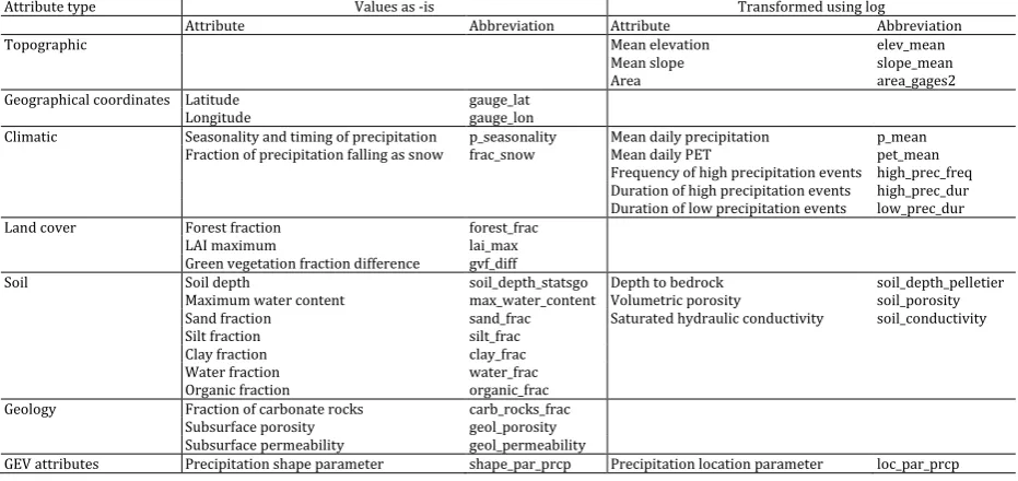
Table 1. Attributes and respective abbreviations of the 671 basins in Addor et al. (2017b) used as predictor variables. The GEV attributes were estimated in the present study. A detailed description of the attributes can be found in Appendix A.
Attribute type Values as -is Transformed using log
Attribute Abbreviation Attribute Abbreviation
Topographic Mean elevation elev_mean
Mean slope slope_mean
Area area_gages2
Geographical coordinates Latitude gauge_lat
Longitude gauge_lon
Climatic Seasonality and timing of precipitation p_seasonality Mean daily precipitation p_mean Fraction of precipitation falling as snow frac_snow Mean daily PET pet_mean
Frequency of high precipitation events high_prec_freq Duration of high precipitation events high_prec_dur Duration of low precipitation events low_prec_dur
Land cover Forest fraction forest_frac
LAI maximum lai_max
Green vegetation fraction difference gvf_diff
Soil Soil depth soil_depth_statsgo Depth to bedrock soil_depth_pelletier
Maximum water content max_water_content Volumetric porosity soil_porosity Sand fraction sand_frac Saturated hydraulic conductivity soil_conductivity
Silt fraction silt_frac
Clay fraction clay_frac
Water fraction water_frac
Organic fraction organic_frac
Geology Fraction of carbonate rocks carb_rocks_frac Subsurface porosity geol_porosity Subsurface permeability geol_permeability
GEV attributes Precipitation shape parameter shape_par_prcp Precipitation location parameter loc_par_prcp
9
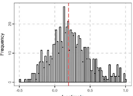
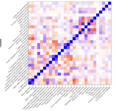
categorical variable; still, it was ranked very low, i.e. 15th in overall), while their inclusion in the linear model was not possible in the testing procedure. The latter is again due to the appearance of missing values in the cross-validation procedure (see Section 2.2.4). Some variables were not considered, because they were highly correlated (correlations higher than 0.9) with other variables; therefore, the inclusion of both variables would not increase the performance of the fitted models. These variables are presented in Table 2 under the term collinearity. From the remaining dataset, basins with more than 100 missing daily streamflow values in the period 1980−2013 or with at least one missing attribute were omitted. The maximum likelihood estimates (Coles 2001, pp. 55, 56) of the parameters of eq. (1) for the annual block maxima of daily streamflow and precipitation were calculated and they were named GEV attributes in Table 1. In particular, the maximum likelihood estimates were obtained using the SpatialExtremes R package (Ribatet 2018). Basins with k ≥ 1 (k denotes the estimate of the shape parameter from hereinafter) were omitted, since E[x] (i.e. the first moment) is not defined for k ≥ 1 (Dey et al. 2016). Here x denotes the GEV random variable that models the streamflow annual block maxima. The 591 remained basins are presented in Figure 1, while the histogram of the k estimates is presented in Figure 2. The correlogram of the remained predictor variables is presented in Figure 3.
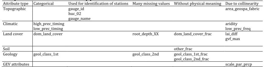
Table 2. Abbreviations of the attributes of the 671 basins in Addor et al. (2017b) not included in the analysis for reasons explained in the heading of the Table. The GEV attributes were estimated in the present study. The names of the attributes and a detailed description can be found in Appendix A.
Attribute type Categorical Used for identification of stations Many missing values Without physical meaning Due to collinearity
Topographic gauge_id area_geospa_fabric
huc_02 gauge_name
Climatic high_prec_timing aridity
low_prec_timing low_prec_freq
Land cover dom_land_cover root_depth_XX dom_land_cover_frac lai_diff
gvf_max
Soil other_frac
Geology geol_class_1st geol_class_2nd geol_class_1st_frac
geol_class_2nd_frac
10
Figure 1. The 591 basins examined and their estimated streamflow GEV shape parameter (or k estimates).
11
Figure 3. Correlations between the predictor variables included in the analysis (see also Table 1).
2.2 Methods
We used two algorithms (i.e. linear models and random forests) to predict the k parameter as a response to the attributes of the basin. All computations were performed using the R Programming Language (R Core Team 2018) and the contributed packages mentioned in Appendix C. Several other utilities accompanying linear models and random forests were implemented in the present study. These are presented in the following.
2.2.1 Linear models
12
importance for a number of predictor variables higher than a specific value depending on the specific case is not substantial. On the other hand, important predictor variables should not be removed. To this end stepwise backward regression, in which each fitted model is evaluated with the Akaike information criterion (AIC; Akaike 1974), can be used and unimportant predictor variables can be removed according to an automatic
procedure. Stepwise backward regression is performed by implementing the olsrr R
package (Hebbali 2018).
Linear models including interactions are also examined. In common statistical literature, the term interaction denotes the influence of the product of two or more predictor variables to the response. This approach differentiates from the usual approach in which the effects of the predictor variables are additive. The concept of interaction differs from the concept of confounding, which in Gaussian-based settings is equivalent with correlation (Boulesteix et al. 2015). Interactions between two predictor variables x1 and x2 are notated with x1 : x2. The notation x1 × x2 := x1 : x2 + x1 + x2 is used to denote that additive terms are included in the interaction term.
Ranking the relative importance of the predictor variables in the linear model is crucial for understanding how the predictor variables affect the dependent variable (Grömping 2007a). The LMG relative importance metric (abbreviation of Lindeman, Merenda, and
Gold 1980 who introduced the metric) is here used through the relaimpo R package
(Grömping 2007b, 2018). The LMG metric decomposes the r2 values of the fitted model into contributions from different predictor variables (see Grömping 2007a). While there
are many methods to decompose r2, the LMG metric is amongst the most credible ones
(Grömping 2007a, b). For instance, LMG is invariant to the ordering of the predictor variables in the linear model, unlike the most frequently used Analysis of Variance (ANOVA).
13
Despite omitting highly correlated predictor variables in the examined dataset (see Section 2.1), the remaining variables still have some residual correlation. A suitable metric to examine the influence of the correlated variables in the linear model (also
termed collinearity) is the Variance Inflation Factor (VIF, O'Brien 2007). Let v2i represent
the proportion of variance of the ith predictor variable, which is associated with the other
predictor variables in the model. The VIF metric is defined by 1/(1 – v2i) and intuitively is
interpreted as the effect of v2i on the variance of the estimated regression coefficient of the
ith predictor variable (O'Brien 2007). As a rule of thumb, common unacceptable values of the VIF metric are those that are higher than 10, albeit in some studies the limit reduces to 4. However, these rules should not be strictly applied (see the discussion in O'Brien 2007) and models including predictor variables with VIF higher than 10 can become acceptable.
2.2.2 Random forests
Random forests are a machine learning algorithm with a few parameters to optimize, while they are simple with high predictive accuracy and successful implementation in practical problems and forecasting competitions (Scornet et al. 2015; Biau and Scornet 2016). A detailed presentation of random forests and related concepts and terminology oriented to the purpose of our study is available in Appendix B. Random forests are used
here for regression by implementing the randomForest R package (Liaw and Wiener
2002; Breiman et al. 2018). The algorithm has four hyperparameters (see also Appendix B). When increasing the number of trees hyperparameter, predictions become more accurate at the cost of increasing the computational time (Oshiro et al. 2012). The number of trees is set equal to 1 000 in the present study, since the gain in the predictive performance of the algorithm would be small by adding more trees (e.g. Probst and Boulesteix 2018). The other hyperparameters were also not optimized, because their predictive performance using their default values is similar to the predictive performance of the optimized algorithms, while the gain in computational time is high when optimization is not performed (see e.g. Biau and Scornet 2016).
14
reason, the examination of both algorithms is useful. An important remark is that in contrast to the linear model, random forests are robust to the inclusion of many and non-important predictor variables (Díaz-Uriarte and De Andres 2006); thus, including all predictor variables would hardly affect the predictive performance of the model.
The permutation importance, which measures the mean increase of the prediction Mean Squared Error on the out-of-bag portion of the data after permuting each predictor variable in the trees of the trained model, was used as relative variable importance metric.
It was computed by implementing the randomForest R package. Relevant details are
presented in the documentation of Breiman et al. (2018) (see also Appendix B).
2.2.3 Naïve prediction
The predictive performance of the regression models is compared to the naïve approach. In the latter, the predicted value of the k parameter is equal to its median value from the training sample in the 10-fold cross validation (see Section 2.2.4). Naïve prediction is used as worst-case benchmark.
2.2.4 10-fold cross validation
To test the predictive performance of the regression models (naïve, linear or random forests) 10-fold cross validation is performed (Kuhn and Johnson 2013, pp. 69–71). In particular, the sample is randomly divided into ten equal sized subsamples. The model is trained in nine subsamples and tested in the remaining one, while the procedure is repeated ten times. The Root Mean Square Error (RMSE), the Pearson’s r and the slope of the regression line between the predicted and testing values are the metrics used for the assessment of the predictive performance of the regression models.
15
2.2.5 The proposed framework
The proposed framework consists of the following sequential steps.
Step 1: Application of stepwise backward linear regression to the whole dataset. Let n1 be the number of the retained predictor variables.
Step 2: Computation of LMG importance metrics for the retained predictor variables of Step 1.
Step 3. Computation of relative importance metrics for random forests when using all predictor variables.
Step 4. 10-fold cross validation with random forests using (a) all predictor variables (b) all predictor variables excluding geographical coordinates (c) the groups of predictor variables defined in Table 1.
Step 5. Again 10-fold cross validation with random forests. In this new model, training the most important variable according to the variable importance metric for random forests is included. Subsequently, the cross validation is repeated by adding one predictor variable at the time according to their importance. The procedure terminates when the performance of the last trained model is similar to the performance of the model that uses all predictor variables.
Step 6. The same procedure (procedure of Step 5) is repeated with the linear model, but here it terminates when using all predictor variables of Step 1. The LMG variable importance metric is used for ranking the variable importance and selecting the additional predictor variable in each iteration. Furthermore, AIC and BIC are computed for each fitted model.
Step 7. 10-fold cross validation is also performed for the naïve method.
Step 8. From the results of the steps 4–7 we understand (a) the performance of the models, (b) the importance of variables using two available metrics and (c) how the inclusion of more predictor variables increases (or decreases) the predictive performance of the models.
16
to first examine interactions between climatic attributes, since (as will be shown in the following Sections, when following steps 1–3) they are found to be the most important in the predictive model.
Step 10. Finally (and hopefully), a parsimonious (i.e. with few predictor variables) linear model with interacting terms and high predictive performance (slightly worse than the best random forest model) appears. According to the criteria set, other linear models may slightly outperform the proposed model; however, they are too complicated, because they include many predictor variables. The selected linear model is investigated by computing VIF and p-values.
2.2.6 Some remarks on the proposed framework
Some remarks on the steps of the procedure of the proposed framework are presented here:
Steps 1–3: Regarding the selection of important variables, we mention that, when many predictor variables (i.e. more than approximately 20 in our dataset) are included in the model fitting, the LMG cannot be computed in a regular home PC. Random forests are used in predictive modelling, in which variable selection is required through e.g. recursive procedures. In this case, these procedures are informative and can accompany other predictive models (Boulesteix et al. 2012). Variable importance, when including all predictor variables in the regression model, can be computed in a reasonable time if random forests are implemented. Consequently, variable importance computation with random forests is convenient when compared, e.g. with linear models, due to computational speed advantages. Therefore, a proposed strategy by Ziegler and König (2014) is to select important predictor variables using random forests in the beginning and, subsequently, use more computationally intensive methods (e.g. related to linear models) in the following. Here we decided to remove predictor variables in the linear model and then compare the results with the random forests. In our opinion, this strategy is equally reasonable.
17
decision is based on the assumption that the importance of non-important variables is randomly distributed around zero.
Steps 4, 5: Regarding the selection of random forests as best case benchmark predictive model we mention that random forests are fast, flexible, robust, they can cope with high-dimensional data (i.e. few observations but many predictor variables), highly correlated variables, interactions between predictor variables, non-linear relationships between the response and the predictor variables and are non parametric, i.e. the specification of a statistical model is not required (Boulesteix et al. 2012; Ziegler and König 2014). Correlated variables have a very slight influence in the predictive performance of random forests (Boulesteix et al. 2012). They were found to outperform other methods, as well as hydrological models in hydrological signatures predictions (Zhang et al. 2018).
Variable importance metrics can be affected by strongly correlated variables; therefore, in some cases a few representative predictor variables should be selected. However, excluding all correlated variables is also not recommended, since information is lost. In this case, there should be some compromise between all options (Boulesteix et al. 2012). Removal of confounding can be done by adding the effect of the confounder separately in e.g. a multiple regression model. In this case, if for instance the effects of both confounders are positive, then the coefficients of the predictor variables are expected to be smaller compared to the case in which one of them is present (Boulesteix et al. 2015).
Step 10: We mention that the selection of a useful model is not only a matter of objectivity. As mentioned by Gelman and Hening (2017) “practitioners must apply their
subjective judgement in the choice of what method to use, what assumptions to invoke and what data to include in their analyses”. For instance, the choice of a linear model with a
18 3. Application
3.1 Application of linear model
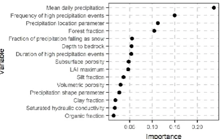
We applied a linear model to better understand the effect of the predictor variables of Table 1. In this application, we excluded the geographical coordinates, because this would not have a physical meaning, unless spatial models such as kriging were used in the modelling procedure. When including all variables of interest of Table 1 the computation of the LMG metric was not possible due to the high computational cost (see Section 2.2.6). Therefore, by applying the stepwise backward regression we excluded some variables not important for the prediction of k. The remaining variables, as well as their respective LMG metric values, are presented in Figure 4.
Figure 4. LMG relative importance metric for the predictor variables presented in the y-axis when a linear model is used to predict the shape parameter.
3.2 Application of random forests
19
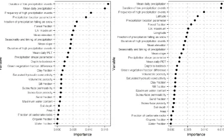
Figure 5. Variable importance of explanatory variables of interest in Table 1 (the geographical coordinates are excluded in the left and included in the right) when random forests are applied to the dataset of the 591 stations to predict the shape parameter. The variable importance of a particular variable is the percentage of increase in mean square error observed in out-of-bag (OOB) prediction when this variable is randomly permuted (Breiman et al. 2018, see also Appendix B).
The ranking of the variables with respect to their importance is slightly different in the two cases. When excluding the geographical coordinates, the most important variables are the mean daily precipitation and the duration of low precipitation events. They are followed by the frequency of high precipitation events and the precipitation GEV location parameter. The fraction of precipitation falling as snow and the forest fraction are also important variables. We note here again that variable importance metrics rank the predictor variables, but the values of the metrics are less informative (see Section 2.2.6). Therefore, they should be combined with the predictive performance of the models, to understand their absolute contribution to the k parameter. This examination follows in Sections 3.3 and 3.4. Here we mention that the increase in the performance of the random forest based predictive models flattens after including 7 to 8 predictor variables (see again Section 2.2.6), and this is the criterion used here to characterize a predictor variable as important.
20
the earlier mentioned ones. The maximum monthly mean of the leaf area index (LAI maximum) also becomes an important variable.
3.3 General results
In both models, the most important variables are climatic indices (the GEV parameters of precipitation can also be considered as climatic indices). Important variables of other types are the forest fraction, the LAI maximum, the catchment mean elevation, the catchment mean slope and the depth to bedrock depending on the employed model. Τhe duration of low precipitation events was excluded when applying the stepwise backward regression, albeit it is an important variable in the random forest model.
21
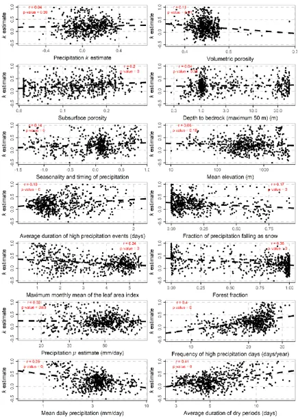
Figure 6. Scatterplots of the shape parameter and predictor variables of interest. The line is obtained by the linear regression of the shape parameter with the predictor variable. The p-values and Pearson’s r of the linear model are also depicted.
22
models are evaluated using 10-fold cross validation. The models are trained on the 90% of the data and predict k for the remaining 10% of the data. The procedure is repeated 10 times, while the respective metrics are equal to the mean of their 10 values obtained from the 10-fold cross-validation. Optimal values of the RMSE should be near 0, of Pearson’s r should be near 1 and the slope should be near 1. When the slope is equal to 1, the regression line between the predicted and the real values of k makes an angle of 45° with the x-axis.
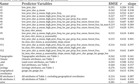
The rf1–rf11 models include important predictor variables based on Figure 5. The first model includes the most important predictor variable, while an important predictor variable based on the ranking of Figure 5 is added in the model at each step. The rf12 model includes the predictor variables of the rf11model and the geographical coordinates. The topographic, climate, land, soil, geology and geographical coordinates random-forest-based models include the respective variables defined in Table 1. The reason is that we aim to understand how each particular type of attributes influences the
k parameter. Two additional models, which are based on random forests and include all
predictor variables of Figure 5, are examined with the aim to estimate the best prediction of k using the available data. The results of the naïve model are also presented in Table 3.
Table 3. Mean model errors (see Section 2.2.4) on the test set of the 10-fold cross-validation for predicting the shape parameter for each method and metric using random forests. The naïve method is also presented.
Name Predictor Variables RMSE r slope
rf1 low_prec_dur 0.291 0.284 0.196
rf2 low_prec_dur, p_mean 0.242 0.518 0.338
rf3 low_prec_dur, p_mean, high_prec_freq 0.233 0.552 0.347
rf4 low_prec_dur, p_mean, high_prec_freq, loc_par_prcp 0.227 0.577 0.363 rf5 low_prec_dur, p_mean, high_prec_freq, loc_par_prcp, frac_snow 0.223 0.599 0.368 rf6 low_prec_dur, p_mean, high_prec_freq, loc_par_prcp, frac_snow, forest_frac 0.221 0.607 0.383 rf7 low_prec_dur, p_mean, high_prec_freq, loc_par_prcp, frac_snow, forest_frac, lai_max 0.219 0.620 0.384 rf8 low_prec_dur, p_mean, high_prec_freq, loc_par_prcp, frac_snow, forest_frac,
lai_max, elev_mean, 0.217 0.628 0.391
rf9 low_prec_dur, p_mean, high_prec_freq, loc_par_prcp, frac_snow, forest_frac, lai_max, elev_mean, p_seasonality
0.215 0.634 0.404 rf10 low_prec_dur, p_mean, high_prec_freq, loc_par_prcp, frac_snow, forest_frac,
lai_max, elev_mean, p_seasonality, slope_mean 0.215 0.632 0.401 rf11 low_prec_dur, p_mean, high_prec_freq, loc_par_prcp, frac_snow, forest_frac,
lai_max, elev_mean, p_seasonality, slope_mean, high_prec_dur 0.216 0.632 0.397 rf12 low_prec_dur, p_mean, high_prec_freq, loc_par_prcp, frac_snow, forest_frac,
lai_max, elev_mean, p_seasonality, slope_mean, high_prec_dur, gauge_lat, gauge_lon 0.214 0.641 0.409
Topographic Topographic attributes, see Table 1 0.262 0.355 0.161
Climate Climatic attributes, see Table 1 0.218 0.621 0.390
Land Land cover attributes, see Table 1 0.243 0.500 0.252
Soil Soil attributes, see Table 1 0.260 0.362 0.157
Geology Geology attributes, see Table 1 0.276 0.241 0.091
Geographical
coordinates gauge_lat, gauge_lon 0.224 0.615 0.396
All attributes 1 All attributes of Table 1, excluding geographical coordinates 0.214 0.641 0.387
All attributes 2 All attributes of Table 1 0.213 0.642 0.393
23
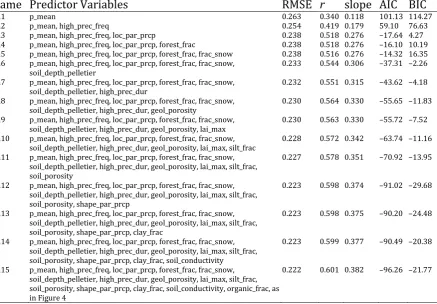
The sequence of fitted linear models is presented in Table 4. The lm1–lm16 models include predictor variables according to their ranking of Figure 4. The AIC and BIC values of the linear models when fitted to the whole dataset are also presented.
Table 4. Mean model errors (see Section 2.2.4) on the test set of the 10-fold cross-validation for predicting the shape parameter for linear models. AIC and BIC are computed when the linear model is fitted to the whole dataset.
Name Predictor Variables RMSE r slope AIC BIC
lm1 p_mean 0.263 0.340 0.118 101.13 114.27
lm2 p_mean, high_prec_freq 0.254 0.419 0.179 59.10 76.63
lm3 p_mean, high_prec_freq, loc_par_prcp 0.238 0.518 0.276 –17.64 4.27 lm4 p_mean, high_prec_freq, loc_par_prcp, forest_frac 0.238 0.518 0.276 –16.10 10.19 lm5 p_mean, high_prec_freq, loc_par_prcp, forest_frac, frac_snow 0.238 0.516 0.276 –14.32 16.35 lm6 p_mean, high_prec_freq, loc_par_prcp, forest_frac, frac_snow,
soil_depth_pelletier
0.233 0.544 0.306 –37.31 –2.26 lm7 p_mean, high_prec_freq, loc_par_prcp, forest_frac, frac_snow,
soil_depth_pelletier, high_prec_dur 0.232 0.551 0.315 –43.62 –4.18 lm8 p_mean, high_prec_freq, loc_par_prcp, forest_frac, frac_snow,
soil_depth_pelletier, high_prec_dur, geol_porosity 0.230 0.564 0.330 –55.65 –11.83 lm9 p_mean, high_prec_freq, loc_par_prcp, forest_frac, frac_snow,
soil_depth_pelletier, high_prec_dur, geol_porosity, lai_max 0.230 0.563 0.330 –55.72 –7.52 lm10 p_mean, high_prec_freq, loc_par_prcp, forest_frac, frac_snow,
soil_depth_pelletier, high_prec_dur, geol_porosity, lai_max, silt_frac 0.228 0.572 0.342 –63.74 –11.16 lm11 p_mean, high_prec_freq, loc_par_prcp, forest_frac, frac_snow,
soil_depth_pelletier, high_prec_dur, geol_porosity, lai_max, silt_frac, soil_porosity
0.227 0.578 0.351 –70.92 –13.95
lm12 p_mean, high_prec_freq, loc_par_prcp, forest_frac, frac_snow, soil_depth_pelletier, high_prec_dur, geol_porosity, lai_max, silt_frac, soil_porosity, shape_par_prcp
0.223 0.598 0.374 –91.02 –29.68
lm13 p_mean, high_prec_freq, loc_par_prcp, forest_frac, frac_snow, soil_depth_pelletier, high_prec_dur, geol_porosity, lai_max, silt_frac, soil_porosity, shape_par_prcp, clay_frac
0.223 0.598 0.375 –90.20 –24.48
lm14 p_mean, high_prec_freq, loc_par_prcp, forest_frac, frac_snow, soil_depth_pelletier, high_prec_dur, geol_porosity, lai_max, silt_frac, soil_porosity, shape_par_prcp, clay_frac, soil_conductivity
0.223 0.599 0.377 –90.49 –20.38
lm15 p_mean, high_prec_freq, loc_par_prcp, forest_frac, frac_snow, soil_depth_pelletier, high_prec_dur, geol_porosity, lai_max, silt_frac, soil_porosity, shape_par_prcp, clay_frac, soil_conductivity, organic_frac, as in Figure 4
0.222 0.601 0.382 –96.26 –21.77
24
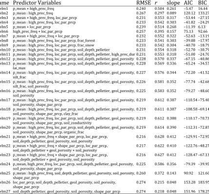
As representative model we select the newlm17 one (further reasoning along with other details can be found later in Section 4.3).
Table 5. Mean model errors (see Section 2.2.4) on the test set of the 10-fold cross-validation for predicting the shape parameter for linear models with interactions. AIC and BIC are computed when the linear model is fitted to the whole dataset. Here a : b denotes interaction while a × b := a + b + a : b (includes interactions and additive effects, see Section 2.2.1).
Name Predictor Variables RMSE r slope AIC BIC
newlm1 p_mean × high_prec_freq 0.240 0.504 0.261 –5.47 16.44
newlm2 p_mean : high_prec_freq 0.267 0.297 0.089 120.12 133.27
newlm3 p_mean × high_prec_freq, loc_par_prcp 0.231 0.553 0.317 –53.44 –27.15 newlm4 p_mean : high_prec_freq, loc_par_prcp 0.233 0.542 0.303 –41.82 –24.29
newlm5 p_mean + loc_par_prcp 0.239 0.514 0.268 –11.39 6.13
newlm6 high_prec_freq + loc_par_prcp 0.257 0.395 0.157 75.13 92.66 newlm7 p_mean × high_prec_freq × loc_par_prcp 0.232 0.552 0.322 –52.63 –13.19 newlm8 p_mean : high_prec_freq, loc_par_prcp, frac_forest 0.233 0.541 0.303 –39.88 –17.97 newlm9 p_mean : high_prec_freq, loc_par_prcp, frac_snow 0.233 0.542 0.304 –40.70 –18.79 newlm10 p_mean : high_prec_freq, loc_par_prcp, soil_depth_pelletier 0.231 0.554 0.318 –52.70 –30.79 newlm11 p_mean : high_prec_freq, loc_par_prcp, soil_depth_pelletier, high_prec_dur 0.231 0.553 0.318 –51.00 –24.70 newlm12 p_mean : high_prec_freq, loc_par_prcp, soil_depth_pelletier, geol_porosity 0.228 0.570 0.337 –67.15 –40.86 newlm13 p_mean : high_prec_freq, loc_par_prcp, soil_depth_pelletier, geol_porosity,
lai_max 0.228 0.569 0.336 –65.24 –34.57
newlm14 p_mean : high_prec_freq, loc_par_prcp, soil_depth_pelletier, geol_porosity,
silt_frac 0.227 0.576 0.344 –72.20 –41.52
newlm15 p_mean : high_prec_freq, loc_par_prcp, soil_depth_pelletier, geol_porosity,
silt_frac, soil_porosity 0.226 0.581 0.352 –77.74 –42.68
newlm16 p_mean : high_prec_freq, loc_par_prcp, soil_depth_pelletier, geol_porosity,
soil_porosity 0.225 0.583 0.352 –79.27 –48.60
newlm17 p_mean : high_prec_freq, loc_par_prcp, soil_depth_pelletier, geol_porosity,
soil_porosity, shape_par_prcp 0.219 0.612 0.387 –110.54 –75.48 newlm18 p_mean : high_prec_freq, loc_par_prcp, soil_depth_pelletier, geol_porosity,
soil_porosity, shape_par_prcp, clay_frac 0.219 0.611 0.387 –108.58 –69.14 newlm19 p_mean : high_prec_freq, loc_par_prcp, soil_depth_pelletier, geol_porosity,
soil_porosity, shape_par_prcp, soil_conductivity 0.219 0.612 0.388 –110.17 –70.73 newlm20 p_mean : high_prec_freq, loc_par_prcp, soil_depth_pelletier, geol_porosity,
soil_porosity, shape_par_prcp, organic_frac
0.219 0.614 0.390 –112.31 –72.87 newlm21 p_mean × high_prec_freq × shape_par_prcp, loc_par_prcp,
soil_depth_pelletier, geol_porosity, soil_porosity 0.216 0.628 0.412 –129.91 –72.95 newlm22 p_mean × high_prec_freq × shape_par_prcp, loc_par_prcp,
soil_depth_pelletier × geol_porosity × soil_porosity 0.217 0.622 0.410 –122.76 –48.27 newlm23 p_mean × high_prec_freq × shape_par_prcp, loc_par_prcp,
soil_depth_pelletier × geol_porosity, soil_porosity 0.216 0.627 0.412 –128.47 –67.13 newlm24 p_mean, high_prec_freq, loc_par_prcp, soil_depth_pelletier, geol_porosity,
soil_porosity, shape_par_prcp 0.225 0.586 0.356 –79.39 –39.95 newlm25 p_mean : high_prec_freq, soil_depth_pelletier, geol_porosity, soil_porosity,
shape_par_prcp 0.260 0.372 0.143 90.92 121.60
newlm26 loc_par_prcp, soil_depth_pelletier, geol_porosity, soil_porosity,
shape_par_prcp 0.274 0.215 0.048 153.28 183.95
newlm27 soil_depth_pelletier, geol_porosity, soil_porosity, shape_par_prcp 0.274 0.218 0.048 151.96 178.25 To understand how differences in the RMSE, which can be perceived as small, can largely influence predictive uncertainties, we compute prediction intervals for the 500-year floods for all basins. The T-500-year flood is defined by (Dey et al. 2016; Tyralis and Langousis 2018):
qT = μ + (σ/k) ( (–log(1–1/T))–k – 1) (2)
25
Section 4.3). The difference in the mean RMSE of the 10-fold cross validation between the two models is 0.014. The p-value of the WSRT is equal to 0.075, i.e. it is lower than the significance level 0.10, indicating that the difference is significant. Since the focus here is to isolate the influence of the k parameter, the μ and σ parameters are set equal to their known values (i.e. the maximum likelihood estimates). Then 10-fold cross validation is implemented for both linear models and 95% prediction intervals for k are computed at the independent sets using the lm R function. Since the quantile is an increasing function of k, as can be derived by eq. (2), 95% prediction intervals can be obtained for q500 by simply substituting k in eq. (2) with its prediction limits. Coverage probabilities for newlm17 and newlm4 are equal to 0.949 and 0.956 respectively. However, the prediction intervals of the newlm17 model are considerably narrower compared to those produced by newlm4. In particular, we computed the relative decrease in the width of the prediction interval between the two models in each basin (in the 10 independent test sets of the 10-fold cross validation) according to:
a = (widthnewlm4 – widthnewlm17)/ widthnewlm4 (3)
The mean relative decrease in the sample of all basins is 4.99%, while the histogram of the relative improvements per basin can be found in Figure 7. To understand the difference between the two models, it is mentioned that the mean width of the prediction intervals are 4 785 m3/s and 5 460 m3/s for the newlm17 and newlm4 models respectively, while 500-year floods range up to 20 000 m3/s.
26 3.4 Overview of results
3.4.1 Naïve method
We limit our following discussion mainly to the assessment of the predictive performance with respect to the value of the RMSE reported in Section 3.3. The naïve method serves as a benchmark; therefore, all combinations of predictor variables and all applied models should be assessed based on their relative performance compared to it. The RMSE in the estimation of k when applying the naïve method is equal to 0.281. It could be said informally that the naïve method is equivalent to not using any predictor variables for k in the models introduced, for example, by Northrop (2004).
3.4.2 Linear models
When applying the linear model by adding one variable at a time the increase in performance is small. However, the use of 12 variables (lm12) leads to a performance that is approximately equal to the one of the rf model with the geographical coordinates, i.e. the RMSE is 0.223 (21% increase in performance compared to the naïve method). The use of all predictor variables presented in Figure 4 results in a RMSE of 0.222, while when including 3−5 predictor variables (lm3−lm5) the RMSE becomes 0.238. The increase in performance is 15%. Finally, the inclusion of six predictor variables results in a 17% increase in performance. These values are important benchmarks for understanding the importance of the predictor variables when added in stepwise mode.
3.4.3 Random forests
27
through the predictor variables of rf5. This is important, since the information from the CAMELS dataset can be transferred to geographical coordinates not included in the CONUS, using just five predictor variables.
It is further important to understand how the different types of attributes of the catchments can be used to increase the information for k. The climatic indices result in an RMSE equal to 0.218, which is significantly low compared to the naïve approach, while its difference compared to the optimal model is also very small. The other types of predictor variables (see Table 1) do not seem to be particularly useful for the prediction model. The land cover characteristics seem to improve the performance of the model with an RMSE equal to 0.243. They are followed by the soil and topographic characteristics with RMSE values equal to 0.260 and 0.262 respectively. The improvement using geological characteristics is negligible.
Compared to the naïve approach, the optimal model results in an increase in performance of the RMSE equal to 24%, which is a considerable improvement. The respective improvement in performance when applying the rf5 model is 21%. This improvement is fair as well, if we also consider the fact that it can be achieved by using only five predictor variables.
3.4.4 Summary of results
The mean Pearson’s r in the 10-fold cross-validation is approximately equal to 0.60, while its exact value depends on the combination of predictor variables and the selected model. The patterns of change in performance are similar to the patterns observed for RMSE. Here again, we highlight that in this kind of studies the relative importance compared to naïve methods is of high importance, and therefore the approach should not be exclusively assessed based on criteria related to the absolute performance. A Pearson’s r equal to 0.60 may not be close to 1, yet the improvement is considerable compared to its respective value when explanatory information is not used. The case for the slope of the regression line is also similar. The slope of the naïve method is 0, while it increases to 0.40 for rf12.
28
significance that the most important variables entered firstly in the models are climate indices.
4. Discussion
4.1 Some additional remarks on the experimental design
Shmueli (2010) identifies three modelling perspectives, i.e. predictive, explanatory and descriptive modelling. Breiman (2001) makes a distinction between two cultures in statistical modelling. In the first culture, it is assumed that the data are generated by a statistical model, while in the second culture that the data are modelled by a non-parametric model, since the data mechanism is considered unknown. According to Boulesteix and Schmid (2014) these two approaches are related, i.e. the statistical approach should be preferred when descriptive modelling is required, while non-parametric approaches (termed algorithmic approaches in Breiman 2001) are suitable in the second case. In some cases, it is possible that a statistical model can also perform equally well to an algorithmic model; therefore, it can simultaneously answer questions related to the description of the model and its predictability. If such a model can be found, as is the case here, then it can answer multiple questions.
29
depends on the specific case examined. The latter involves comparison with naïve methods and intercomparison of models with varying number of predictor variables with respect to their predictive performance.
4.2 New findings on the nature of the k parameter
30
study includes a higher number of examined basins and attributes, while the basins represent a large diversity of climate types.
4.3 The final model
Random forests is an algorithm with high predictive performance and an ability to reveal interactions between the predictor variables and non-linear relationships (see Section 2.2.6). Therefore, the here lowest predictive performance of the linear model should be expected. Considering that the improvement of other algorithms is expected to be low compared to random forests, it is reasonable to assume that an optimal benchmark regarding the prediction of k would be a result from the implementation of random forests. Considering also the need for obtaining an interpretable and parsimonious model, a linear model with a small number of predictor variables should be selected in the model. Such a model is the newlm17, which includes five predictor variables and the interaction between other two attributes, when fitted to the sample of the 591 catchments as shown in the next equation:
k = – 2.61 + 0.87 log (precipitation location parameter) – 0.03 log(depth to bedrock) +
0.46 subsurface porosity – 0.66 log(volumetric porosity) + 0.30 precipitation GEV shape parameter – 0.32 log(mean daily precipitation) log(frequency of high precipitation
events) (4)
It is obvious that the newlm17 model has good predictive properties, since it is better than all linear models in Table 4, highlighting the role of interactions. It is also slightly worse compared to the rf8−rf12 random forest models with respect to its predictive performance; however, it is more interpretable and includes less predictor variables. It is also notable that the rate of increase in the predictive performance of random forests decreases rapidly as more predictor variables are added in the models. Therefore, starting from an RMSE equal to 0.291 (rf1 model in Table 3), an intermediate RMSE equal to 0.219 is reached (rf7 in Table 3), while the terminating RMSE is equal to 0.214 (rf14 model in Table 3). A delivered RMSE equal to 0.219, together with a small number of predictor variables and a simple model structure, are good reasons to select the newlm17 model for the given data.
31
acceptable, especially if we consider that their exclusion results in significant decrease in performance. The VIF of the predictor variables were in the range 1−1.5 (1 is the lower limit of VIF). The residuals of the newlm17 model were also found normally distributed according to the Shapiro-Wilk test. The model of eq. (4) uses seven predictor variables and its RMSE was 0.219 in the 10-fold cross-validation, while the Pearson’s r was equal to 0.612. Its adjusted r2 was 0.39 when fitted to the dataset of the 591 catchments. Furthermore, its performance is equal to the one of the rf7 model, which also includes seven predictor variables.
When looking at eq. (4) one sees that k is a decreasing function of the product of mean daily precipitation and frequency of high precipitation events. The inclusion of the interaction played a crucial role in the considerable increase in performance compared to the models that do not include interactions, i.e. the models of Table 4. Additionally, k increases with the location parameter of the GEV distribution of precipitation extremes and with the increase of their shape parameter. The latter seems also sensible, because extreme precipitation should result in streamflow extremes. Lastly, k increases with increasing subsurface porosity and decreases with increasing depth to bedrock and volumetric porosity. To the authors’ knowledge, there is not a theory-driven explanatory model for the relationship between k and geological or soil attributes. However, the benefits of using such model have been shown in Section 3.3 (see Figure 7 and the relevant discussion on the comparison in the predictive performance between newlm4 (which includes the interaction term and the location parameter of precipitation) and newlm17).
5. Conclusions
The shape parameter of the generalized extreme value distribution of daily annual block maxima of streamflow is important because it is related to how extreme the floods are. For this specific reason, it should be attentively examined with the aim to reduce its high impact on uncertainty, when incorporated in statistical models of extremes.
non-32
linear model (random forests), which is herein used as best case prediction algorithm, aiming to validate the proposed linear model. We applied the framework to 591 basins in the contiguous US.
We found that the shape parameter is influenced by the interactions between the mean daily precipitation and the frequency of high precipitation days, the precipitation GEV location parameter and the precipitation GEV shape parameter. It also depends on geological and soil characteristics of the catchment, albeit to a smaller extent.
The RMSE of the linear model in a 10-fold cross-validation scheme was found to be 0.219, i.e. 22% smaller than the RMSE computed for a naïve model, while its adjusted r2 when the model is fitted to the whole dataset is 0.39. Its performance was similar to the more complex benchmark model, i.e. negligible improvements can be found, by further modification of the model. The incorporation of this model into relevant Bayesian frameworks or regression-based models for regional flood frequency analysis may result in considerable reduction of the predictive uncertainties.
Conflicts of interest: The authors declare no conflict of interest.
Appendix A Description of catchment attributes
In Tables A-1-A-6 we describe the attributes of the basins.
Table A-1. Name, location and topographic characteristics (adapted from Addor et al. 2017b).
Attribute Abbreviation Description
Gauge id gauge_id catchment identifier (eight-digit USGS hydrologic unit code)
Region huc_02 region (two-digit USGS hydrologic unit code)
Gauge name gauge_name gauge name, followed by the state
Latitude gauge_lat gauge latitude
Longitude gauge_lon gauge longitude
Mean elevation elev_mean catchment mean elevation
Mean slope slope_mean catchment mean slope
Area area_gages2 catchment area (GAGESII estimate)
33
Table A-2. Climatic indices (adapted from Addor et al. 2017b).
Attribute Abbreviation Description
Mean daily precipitation p_mean mean daily precipitation
Mean daily PET pet_mean mean daily PET, estimated by N15 using Priestley–Taylor
formulation calibrated for each catchment
Aridity aridity aridity (PET / P, ratio of mean PET, estimated by N15 using
Priestley–Taylor formulation calibrated for each catchment, to mean precipitation)
Seasonality and timing of
precipitation p_seasonality seasonality and timing of precipitation (estimated using sine curves to represent the annual temperature and precipitation cycles; positive (negative) values indicate that precipitation peaks in summer (winter); values close to 0 indicate uniform precipitation throughout the year)
Fraction of precipitation
falling as snow frac_snow fraction of precipitation falling as snow (i.e., on days colder than 0°C)
Frequency of high
precipitation events high_prec_freq frequency of high precipitation days (≥ 5 times mean daily precipitation) Duration of high
precipitation events high_prec_dur average duration of high precipitation events (number of consecutive days ≥ 5 times mean daily precipitation) Season of high
precipitation events high_prec_timing season during which most high precipitation days (≥ 5 times mean daily precipitation) occur Frequency of low
precipitation events low_prec_freq frequency of dry days (< 1 mm day
–1)
Duration of low
precipitation events low_prec_dur average duration of dry periods (number of consecutive days < 1 mm day–1) Season of low precipitation
events low_prec_timing season during which most dry days (< 1 mm day
–1) occur
Table A-3. Land cover characteristics (adapted from Addor et al. 2017b).
Attribute Abbreviation Description
Forest fraction forest_frac forest fraction
LAI maximum lai_max Maximum monthly mean of the leaf area index (based on 12
monthly means)
LAI difference lai_diff difference between the maximum and minimum monthly mean
of the leaf area index (based on 12 monthly means) Green vegetation fraction
maximum gvf_max maximum monthly mean of the green vegetation fraction (based on 12 monthly means)
Green vegetation fraction
difference gvf_diff difference between the maximum and minimum monthly mean of the green vegetation fraction (based on 12 monthly means)
Dominant land cover dom_land_cover dominant land cover (Noah-modified 20-category IGBP-MODIS
land cover) Dominant land cover
fraction dom_land_cover_frac fraction of the catchment area associated with the dominant land cover
Root depth root_depth_XX root depth (percentiles XX = 50 and 99 % extracted from a root
34
Table A-4. Soil characteristics (adapted from Addor et al. 2017b).
Attribute Abbreviation Description
Depth to bedrock soil_depth_pelletier depth to bedrock (maximum 50 m)
Soil depth soil_depth_statsgo soil depth (maximum 1.5 m; layers marked as water and
bedrock were excluded)
Volumetric porosity soil_porosity volumetric porosity (saturated volumetric water content
estimated using a multiple linear regression-based on sand and clay fraction for the layers marked as USDA soil texture class and a default value (0.9) for layers marked as organic material; layers marked as water, bedrock, and “other” were excluded)
Saturated hydraulic
conductivity soil_conductivity saturated hydraulic conductivity (estimated using a multiple linear regression-based on sand and clay fraction for the layers marked as USDA soil texture class and a default value (36 cm h–1) for layers marked as organic material; layers marked as water, bedrock, and “other” were excluded)
Maximum water content max_water_content maximum water content (combination of porosity and
soil_depth_statsgo; layers marked as water, bedrock, and “other” were excluded)
Sand fraction sand_frac sand fraction (of the soil material smaller than 2 mm; layers
marked as organic material, water, bedrock, and “other” were excluded)
Silt fraction silt_frac silt fraction (of the soil material smaller than 2 mm; layers
marked as organic material, water, bedrock, and “other” were excluded)
Clay fraction clay_frac clay fraction (of the soil material smaller than 2 mm; layers
marked as organic material, water, bedrock, and “other” were excluded)
Water fraction water_frac fraction of the top 1.5 m marked as water (class 14)
Organic fraction organic_frac fraction of soil_depth_statsgo marked as organic material
(class 13)
Other fraction other_frac fraction of soil_depth_statsgo marked as “other” (class 16)
Table A-5. Geological characteristics (adapted from Addor et al. 2017b).
Attribute Abbreviation Description
Common geologic class geol_class_1st most common geologic class in the catchment
Fraction of common
geologic class geol_class_1st_frac fraction of the catchment area associated with its most common geologic class Second most common
geologic class geol_class_2nd second most common geologic class in the catchment
Fraction of second most
common geologic class geol_class_2nd_frac fraction of the catchment area associated with its second most common geologic class Fraction of carbonate rocks carb_rocks_frac fraction of the catchment area characterized as “carbonate
sedimentary rocks”
Subsurface porosity geol_porosity subsurface porosity
Subsurface permeability geol_permeability subsurface permeability (log10)
Table A-6. GEV attributes.
Attribute Abbreviation Description
Shape parameter of streamflow
extremes shape_par GEV shape parameter estimate of the streamflow annual block maxima
Precipitation location parameter loc_par_prcp GEV location parameter estimate of the precipitation annual block maxima
Precipitation scale parameter scale_par_prcp GEV scale parameter estimate of the precipitation annual block maxima
Precipitation shape parameter shape_par_prcp GEV shape parameter estimate of the precipitation annual
block maxima
Appendix B Random Forests
35
15). RF are a classification and regression algorithm. Here we use it for regression. The algorithm uses regression trees (see Hastie et al. 2018, Chapter 9) and a modification of bootstrap aggregating (bagging). Breiman’s (2001) RF use the CART decision trees (see Hastie et al. 2018, Chapter 9), while other tree versions also exist. Trees have low bias and can model interactions. The idea of bagging is to average many noisy but approximately unbiased models aiming to reduce the variance. Consequently, a good option is to average many trees. The bias of the average of trees is equal to the bias of each tree; however, bagging reduces the variance of the average of trees. Further reduction of the variance is achieved when a modification of bagging is used. In this modification, each tree grows by a random selection of the input variables. The notation mtryis commonly used to denote the number of variables randomly selected at each tree due to the most frequently used software implementation of the algorithm, i.e. the randomForest (Liaw and Wiener 2002; Breiman et al. 2018) R package. The training of the algorithm is performed by minimizing the out-of-bag (oob) error, i.e. the error of the internal (within the training set) cross-validation of the algorithm.
The algorithm needs little tuning, while its performance is very good when using the default parameters, i.e. mtry, the number of trees, the maximum number of terminal nodes
of the trees and the minimum size of terminal nodes. The number of trees is a critical parameter.
Growing a large number of trees results in better predictions but the performance flattens
asymptotically.
Estimation of the variable importance, i.e. the contribution of each input variable in
predicting the response (see Hastie et al. 2018, Chapter 10; see also Grömping 2015) is also
possible with RF. Variable importance of RF is computed by (a) growning a tree, (b) computing
the prediction accuracy of the tree in the oob sample are passed down, (c) randomly permuting
the jth variable in the oob sample and recomputing the prediction accuracy. The variable
importance of the jth variable is equal to the decrease in accuracy after permuting in all trees
and averaging the results. Negative variable importance means that inclusion of the predictor
variables results in decrease of the performance of the algorithm. Positive values indicate
positive contribution in the prediction of the algorithm, while the magnitude of the contribution
is related to the relative contribution of all variables, as estimated from their respective variable