Finite Element Analyses of Single-Edge Bend Specimens for J-R Curve Development

(1)

Scholarship@Western

Electronic Thesis and Dissertation Repository

9-25-2013 12:00 AM

Finite Element Analyses of Single-Edge Bend Specimens for J-R

Curve Development

Yifan Huang

The University of Western Ontario Supervisor

Dr. Wenxing Zhou

The University of Western Ontario

Graduate Program in Civil and Environmental Engineering

A thesis submitted in partial fulfillment of the requirements for the degree in Master of Engineering Science

Follow this and additional works at: https://ir.lib.uwo.ca/etd

Part of the Applied Mechanics Commons, Civil Engineering Commons, Structural Engineering Commons, and the Structural Materials Commons

Recommended Citation Recommended Citation

Huang, Yifan, "Finite Element Analyses of Single-Edge Bend Specimens for J-R Curve Development" (2013). Electronic Thesis and Dissertation Repository. 1671.

https://ir.lib.uwo.ca/etd/1671

This Dissertation/Thesis is brought to you for free and open access by Scholarship@Western. It has been accepted for inclusion in Electronic Thesis and Dissertation Repository by an authorized administrator of

(2)

(Thesis format: Integrated Article)

by

Yifan Huang

Graduate Program in Engineering Science Department of Civil and Environmental Engineering

A thesis submitted in partial fulfillment of the requirements for the degree of

Master of Engineering Science

The School of Graduate and Postdoctoral Studies The University of Western Ontario

London, Ontario, Canada

(3)

ii

Abstract

The fracture toughness resistance curve such as the J-integral resistance curve (J-R curve) is widely used in the integrity assessment and strain-based design of energy pipelines with respect to planar defects (i.e. cracks). Two studies about the development of the J-R curve are carried out and reported in this thesis. In the first study, the plastic geometry factor, i.e. the ηpl factor, used to evaluate J in a J-R curve test based on the single-edge bend (SE(B))

specimen is developed based on the three-dimensional (3D) finite element analysis (FEA). The main finding of this study is that besides the crack length, both the thickness and side grooves of the specimens have observable impacts on the ηpl factor. The ηpl factors obtained

from 3D FEA are different from those obtained from two-dimensional (2D) FEA. The results of this study can improve the accuracy of the experimentally determined J-R curve and facilitate the use of non-standard (e.g. shallow-cracked) SE(B) specimens for the J-R

curves testing. In the second study, 3D FEA is carried out on SE(B) specimens for which the

J-R curves have been experimentally determined to develop the constraint-corrected J-R

curves for X80 grade pipe steels. The constraint parameters considered in this study include

Q, A2, h and Tz. Several different forms of the Q parameter that account for the correction for

the load and/or bending stresses are considered. It is observed that three constraint parameters, namely QBM1, Tz and A2, lead to reasonably accurate constraint-corrected J-R curve for a wide range of crack extension compared with the J-R curves experimentally determined from two shallow cracked SE(B) specimens. On the other hand, the constraint-corrected J-R curve based on constraint parameters QHRR, QBM2 and Qm lead to a relatively

large error of prediction. The approach for constructing the constrain-corrected J-R curve can be used to develop the structure-specific J-R curve based on those obtained from small-scale test specimens to improve the accuracy of the structural integrity assessment.

Keywords

(4)

iii

Co-Authorship

A version of Chapter 2 co-authored by Wenxing Zhou, Enyang Wang and Guowu Shen has been accepted as a technical paper and presented in the 23rd International Offshore and

Polar Engineering Conference (ISOPE 2013) in Anchorage, Alaska between June 30 and

July 5, 2013.

An extended version of Chapter 2 co-authored by Wenxing Zhou and Zijian Yan has been submitted to the International Journal of Pressure Vessels and Piping as a technical paper.

(5)

iv

Dedication

(6)

v

Acknowledgments

My deepest gratitude goes first and foremost to Dr. Wenxing Zhou, my supervisor, for his patient guidance, understanding, encouragement, and most importantly for continuously supporting me with his profound insight throughout this study. He has walked me through all the stages of the writing of this thesis. Without his consistent and illuminating instruction, this thesis could not have reached its present form. It has been a great privilege and joy of being a member of his research group and studying under his guidance and supervision.

I would also like to thank Dr. Ashraf A. El Damatty, Dr. Tim A. Newson and Dr. Robert Klassen for being my examiners and for their constructive advice to this thesis. I would also express my gratitude to Dr. Guowu Shen, senior research scientist at CANMET-MTL and Adjunct Professor in the Department of Civil and Environmental Engineering at Western, for his valuable comments and suggestions during a project in my thesis.

My special thanks to all my colleagues and alumni in our research group: Enyang Wang, Shenwei Zhang, Guoxiong Huang, Ning Zhang, Mohammad Al-Amin, Bernard Kim, Zijian Yan and Hao Qin, for making my graduate life so enjoyable and also for their encouragement and assistances. A friend in need is a friend indeed!

Financial support provided by TransCanada and the Natural Sciences and Engineering Research Council of Canada (NSERC) and by the Faculty of Engineering at Western University is gratefully acknowledged.

(7)

vi

List of Tables

Table 2.1a: The LLD-based ηpl obtained from varieties of 3D FE models for n = 10 materials

... 34

Table 2.2b: The CMOD-based ηpl obtained from varieties of 3D FE models for n = 10 materials ... 34

Table 2.3a: The LLD-based ηpl obtained from varieties of 3D FE models for n = 5 materials ... 35

Table 2.4b: The CMOD-based ηpl obtained from varieties of 3D FE models for n = 5 materials ... 35

Table 2.5: Variation of ηpl with strain hardening exponent for plane-sided model with B/W = 0.5... 36

Table 3.1: Parameters of the experimental J-R curve for SE(B) specimens ... 72

Table 3.2: Constraint parameters for SE(B) specimens ... 72

Table 3.3: Coefficients qi for the constraint-corrected J-R curve ... 73

Table 3.4: Error of the predicted J-R curve for SEB25 ... 73

(11)

x

List of Figures

Figure 1.1: Three typical loading modes in fracture mechanics ... 12

Figure 1.2: Stress field near the crack tip ... 12

Figure 1.3: Schematic of J-integral ... 13

Figure 2.1: Schematic of the plane-sided (PS) and side-grooved (SG) specimens ... 38

Figure 2.2: Determination of the potential energy ... 39

Figure 2.3: Plastic area under the load-displacement curve ... 39

Figure 2.4: Schematic of the estimation of Jpl for growing cracks ... 40

Figure 2.5: Configuration of the finite element model ... 41

Figure 2.6: Schematics of side-grooved finite element model with a/W = 0.5 and B/W = 0.5 ... ... 42

Figure 2.7: Distribution of the effective stress at mid plane in a typical FE model(a/W = 0.5 and B/W = 1) corresponding to the applied displacement of 1.5mm ... 43

Figure 2.8: Variation of ηpl factor corresponding to Jave with normalized Jpl for a representative specimen (plane-sided, a/W = 0.7, B/W = 1 and n = 10) ... 44

Figure 2.9: Variation of the normalized plastic J with normalized plastic area ... 45

Figure 2.10: Variation of ηpl with a/W for n = 10 ... 47

Figure 2.11: Variation of ηpl with a/W for n = 5 ... 49

Figure 3.1: Typical J-R curves from different types of specimens ... 75

Figure 3.2: Analysis procedures for constructing the constraint-corrected J-R curves ... 75

(12)

xi

Figure 3.4: Experimentally determined J-R curves for SE(B) specimens (Shen et al., 2004) ...

... 77

Figure 3.5: FEA model for SE(B) specimen with a/W= 0.42 ... 78

Figure 3.6: Distributions of the local J along the crack front for SE(B) specimens ... 80

Figure 3.7: Distributions of the crack opening stress as a function of distance from the crack tip for SE(B) specimens ... 81

Figure 3.8: Variation of J0.2 and J1.0 with QHRR ... 82

Figure 3.9: Variation of J0.2 and J1.0 with Qm ... 82

Figure 3.10: Variation of J0.2 and J1.0 with QBM1 ... 83

Figure 3.11: Variation of J0.2 and J1.0 with QBM2 ... 83

Figure 3.12: Variation of J0.2 and J1.0 with A2 ... 84

Figure 3.13: Variation of J0.2 and J1.0 with h ... 84

Figure 3.14: Variation of J0.2 and J1.0 with Tz ... 85

Figure 3.15: C2 obtained in Eq. (3.18b) as a function of constraint parameter ... 87

Figure 3.16: Constraint-corrected J-R curves for SE(B) specimens based on QHRR ... 88

Figure 3.17: Constraint-corrected J-R curves for SE(B) specimens based on Qm ... 89

Figure 3.18: Constraint-corrected J-R curves for SE(B) specimens based on QBM1 ... 90

Figure 3.19: Constraint-corrected J-R curves for SE(B) specimens based on QBM2 ... 91

Figure 3.20: Constraint-corrected J-R curves for SE(B) specimens based on A2 ... 92

Figure 3.21: Constraint-corrected J-R curves for SE(B) specimens based on h ... 93

(13)

xii

Figure A.1: The virtual crack extension method in two-dimensional analysis ... 105

Figure A.2: The virtual shift in three-dimensional analysis ... 106

(14)

xiii

List of Nomenclature

A = area under the load-displacement curve

A1 = parameter in the J-A2 solution

A2 = constraint parameter

AC = area of the cracked body

ACMOD = area under the load versus CMOD curve

Ael, Apl = the elastic and plastic component of area under load-displacement curve ALLD = area under the load versus LLD curve

= Plastic area under the load versus LLD curve = Plastic area under the load versus CMOD curve

, ₌_area_of_AB_{Δ Δ} _{in Fig. 2.4}

̅ _{= non-dimensionalized plastic area}

a = crack length

a0 = initial crack length

ai, ai+1 = values of a at step i and step i+1

B = thickness of the specimen

Be = effective thickness of the specimen BN = net thickness of the specimen b = length of the uncracked ligament

bi, bi+1 = values of b at step i and step i+1

C = linearization factor in bending correction of Q CMOD, V = crack mouth opening displacement

C(T) = compact tension

CTOD = crack tip opening displacement

C1, C2 = power-law coefficients of J-R curves

Ci = compliance obtained in the i th loading-unloading sequence

= CMOD-based compliance obtained in the i th loading-unloading sequence = rotation corrected compliance obtained in the i th loading-unloading sequence

ds = the length increment

(15)

xiv

E = elastic modulus

E’ = effective modulus of elasticity EPFM = elastic plastic fracture mechanics

e = error of the J values in the predicted J-R curves

fij = dimensionless function of θ G = energy release rate

h = stress triaxiality parameter

In = integration constant that depends on n J = nonlinear energy release rate

J0.2, J1.0 =J values corresponding to crack extensions of 0.2 and 1.0 mm in a J-R curve

J2 = the second invariant of the deviatoric stress tensor

Jave = the average J value along the crack front Jel = elastic component of J

JIc, KIc = fracture toughness

Jloc = the local J value at each layer along the crack front Jmid = the local J value at the mid-plane of the crack front Jpl = plastic component of J

 = value of Jpl at B or the intermediate value of Jpl between step i and step i+1

  = values of J at step i and step i+1

JΔai = the J values corresponding to a certain crack extensions in a J-R curve ̅ = non-dimensionalized J

K = stress intensity factor

Kc = critical stress intensity factor

k, L = characteristic length that can be simply set equal to 1 mm LEFM = linear elastic fracture mechanics

LLD, Δ = load-line displacement LSY = large scale yielding

M = moment per unit thickness acting at the center of the cross section MBL = modified boundary layer

n = strain hardening exponent

(16)

xv

P, P  = values of P at step i and step i+1

Pl = reference load Q = constraint parameter

QHRR, QSSY = Q parameters based on HRR solution and small scale yielding analysis Qm, QBM = load-dependence modified and bending corrected Q parameters qi = fitting coefficients of the function of C1 and C2

r,θ = coordinates in the polar coordinate system near the crack tip

rp = the size of the plastic zone ahead of the crack tip rw = radius of the blunt crack tip in FEA model S = the span of the specimen

SE(B) = single-edge bend SE(T) = single-edge tension SSY = small scale yielding

s1, s2, s3 = the stress power exponents in the J-A2 solution

sij = the deviatoric stress tensor Ti = traction vectors Tz = out-of-plane constraint parameter

ti = the component or directional cosine of the unit tangent vector along the crack

front as shown in Fig. A.2

U = strain energy

ui = components of the displacement VC = volume of the cracked body Vpl = plastic component of CMOD W = the width of the specimen

w = the strain energy density

Y = general constraint parameter

 = coefficient in the Ramberg-Osgood stress-strain relationship  = arbitrary counterclockwise contour around the crack tip

 = plastic geometry factor used to calculate Jpl for a growing crack

i = values of  at step i

(17)

xvi

Δa1, Δa2 = any two crack extensions

Δel, Δpl = the elastic and plastic component of LLD

Δ , Δ = values of Δpl at step i and step i+1

δij = Kronecker delta

0 = reference strain, ε0 = σ0/E

ij, = total and plastic strain tensor

 = geometry factor used to calculate J

ave = plastic geometry factor corresponding to the average J value along

the crack front

, = LLD-and CMOD- based ave

mid = plastic geometry factor corresponding to the local J value at the mid-plane.

, = LLD-and CMOD- based mid

pl = plastic geometry factor used to calculate plastic component of J

, = LLD-and CMOD- based pl

= value of pl at step i

0 = reference stress

,  = opening stress ahead of the crack tip obtained from the finite element analysis

and HRR solution

e = the von Mises effective stress

h = the hydrostatic stress

ij = stress tensor

ijHRR = stress state obtained in HRR plane-strain solution

ijSSY = stress field corresponding to the small-scale yielding solution

ijref = reference stress state used to determine constraint parameter Q

UTS = ultimate tensile stress

y = yield strength of the material

, ̃  = dimensionless functions of n, θ in the HRR solution  = angular functions in J-A2 solution

(18)

Chapter 1 Introduction

1.1 Background

Pipelines are effective and safe means to transport large quantity of hydrocarbons over a long distance (PHMSA 2012). Recent years have witnessed the rapid developments of the pipeline industry. According to the Canadian Energy Pipeline Association, there are over 100,000 km of oil and gas transmission pipelines in Canada. It is reported that about $85.5 billion worth of hydrocarbons were shipped through the 71,000 km long pipelines regulated by the National Energy Board (NEB) of Canada in 2010 (NEB 2010).

Energy pipelines may contain planar defects, i.e. cracks, in the pipe base metal and weldments due to various causes such as stress corrosion cracking, fatigue and the welding process. The fracture toughness of the pipe steel and weldments is a key input to the structural integrity assessment of pipelines with respect to planar defects. The fracture toughness also governs the tensile strain capacity of the pipeline, which is a critical component of the strain-based design methodology that is being increasingly used to design pipelines subjected to large plastic deformations resulting from, for example, frost heave, thaw settlement and earthquake-induced ground movements.

For ductile materials such as the modern pipe steels, the fracture process is often accompanied by relatively large plastic deformation at the crack tip and considerable crack extension. In this case, the fracture toughness is typically characterized by the so-called fracture toughness resistance curve that is generally represented by either the J -integral resistance curve (J-R curve) or the crack tip opening displacement (CTOD) resistance curve (CTOD-R curve) (Anderson, 2005).

(19)

(Yuan and Brocks, 1998). A high level of constraint results in a low toughness resistance curve, and a low level of constraint results in a high toughness resistance curve (Yuan and Brocks, 1998). Standard SE(B) and C(T) specimens are deeply cracked to ensure high constraint levels at the crack tip such that the corresponding fracture resistance curves represent the lower bound values. On the other hand, the crack tip constraint level for real cracks in pipelines is typically low because real cracks are generally shallow cracks. The application of the fracture resistance curve obtained from high-constraint specimens to low-constraint real structures may lead to overly conservative design and assessment. This is known as the fracture toughness transferability issue.

Over the last decade, non-standard test specimens such as single-edge notched tensile (SE(T)) and shallow-cracked SE(B) specimens have been investigated to address the fracture toughness transferability (e.g. Dodds et al., 1997). Research (Zhu and Jang, 2001) has also been carried out to develop the so-called constrain-corrected J-R curves, i.e. the J-R curve parameterized by commonly used constraint parameters Q or A2 (O’Dowd and Shih, 1991; Yang et al., 1993a and 1993b).

1.2 Fundamentals of Fracture Mechanics

1.2.1 Linear Elastic Fracture Mechanics

Fracture mechanics can be separated into two main domains: the linear elastic fracture mechanics (LEFM) and the elastic plastic fracture mechanics (EPFM) (Anderson, 2005). LEFM attempts to describe the fracture behavior of a material when the plastic deformation is confined to a small region surrounding the crack tip, known as the small scale yielding (SSY) condition. On the other hand, EPFM applies to the large scale yielding (LSY) where significant plasticity in the vicinity of the crack tip is considered.

(20)

loading because it is the most critical fracture mode for ductile metals. All the discussions thereafter are with respected to the Mode I loading.

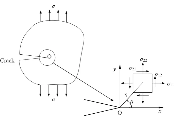
Consider an isotropic linear elastic body containing a crack as illustrated in Fig. 1.2. Define a polar coordinate system with the origin located at the crack tip. The stress field at the crack tip can be written as (Irwin, 1957; Williams, 1957):

 

0 lim 2 ij ij r K f r      

 _ _ (1.1)

where σij1 is the stress tensor; r and θ are coordinates defined in Fig. 1.2; fij is a

dimensionless function of θ, and K is the so-called stress intensity factor in the unit of force/area×(length)0.5. Equation (1.1) describes a stress singularity at the crack tip, because σij approaches infinity as r→0. The stress intensity factor completely defines the

amplitude of the stress singularity; that is, the stresses, strains and displacements near the crack tip can be completely determined given K (Anderson, 2005).

This single-parameter characterization by K relies on satisfaction of the SSY condition, which requires the zone of plastic deformation to be contained well within the singularity fields (Hutchinson, 1983). The size of the plastic zone ahead of the crack tip, rp, can be

approximately calculated using the following equation (Hutchinson, 1983):

2 2 1 plane strain 3 1 plane stress  _ _  __ __                 _ _     y p y K r K

 

(1.2) 1

(21)

where σy is the yield strength. The ASTM standard for experimentally determining the

linear elastic plane strain fracture toughness of metallic materials, ASTM E399 (ASTM, 2013), requires the crack length and uncracked ligament of the test specimen to be not less than 25rp at the point of fracture to satisfy SSY. Generally speaking, SSY is

considered reasonable if the applied load is less than half the limit load at which plastic yielding extends throughout the uncracked ligament (Hutchinson, 1983). In SSY, the energy release rate G, defined as the rate of decrease in the potential energy with a unit increase in the crack area (Irwin, 1956), can be related to the stress intensity factor K as follows:

2 2

2

(1 )

plane strain 1

plane stress _  _{} _ 

 

   

K E G

K E



(1.3)

where ν is Poisson’s ratio and E denotes the elastic modulus.

For a given material at a given temperature, there exists a critical stress intensity factor,

Kc , associated with the onset of crack growth under the monotonic loading (Hutchinson,

1983). In particular, the critical stress intensity factor in mode I, plane-strain condition is called the fracture toughness of the material at the given temperature and denoted by KIc. KIc is expected to be a material property (Broek, 1986). To ensure the plane-strain

condition in the fracture toughness test, ASTM E399 (ASTM, 2013) also requires the thickness of the test specimen to be at least 25rp.

For highly brittle materials, cracks will run dynamically once K reaches KIc, and KIc

(22)

1.2.2 Elastic Plastic Fracture Mechanics

Linear elastic fracture mechanics (LEFM) is invalid when the fracture processes are accompanied by significant plastic deformation at the crack tip (Anderson, 2005). As a rough approximation, the application of LEFM becomes questionable if the applied load is greater than one half of the load at which full plastic yielding occurs (Hutchison, 1983). To characterize the fracture behavior of ductile materials with medium-to-high toughness, the elastic plastic fracture mechanics is required.

Before further discussions of the elastic plastic fracture mechanics, it is necessary to introduce some fundamentals of the theory of plasticity. There are two main theories of plasticity based on two different constitutive relations. The incremental (or flow) theory of plasticity employs the formulations relating increments of stress and strain, whereas the deformation theory of plasticity employs the formulations relating the total stress and strain. The incremental theory of plasticity is loading-path-dependent, whereas the deformation theory of plasticity is loading-path-independent. Under the monotonic and proportional loading condition, the deformation theory of plasticity is equivalent to the incremental theory of plasticity.

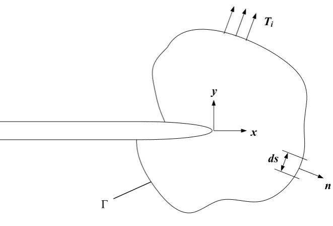
The J-integral proposed by Rice (1968) is perhaps the most important concept in EPFM (Anderson, 2005). Consider a two-dimensional cracked body (see Fig. 1.3) characterized by the deformation theory of plasticity (i.e. small strain kinematics and nonlinear elastic constitutive model) with an arbitrary counterclockwise path (Γ) around the crack tip. The

J-integral or J is defined as

i i

u

J wdy T ds

x





 

 _   _



 



(1.4)

where ui and Ti are components of the displacement and traction vectors, respectively (i =

1, 2 or 3); w is the strain energy density, and ds is the length increment along the contour

(23)

 

,

 

₀ij

ij ij ij

w w x y w  

_

  d (1.5)

i ij j

T  n (1.6)

where εij (i, j = 1, 2, or 3) is the strain tensor, and nj is the component of the unit normal

vector to Γ. Rice (1968) showed that the value of J is independent of the integration path, i.e. Γ, around the crack tip. Therefore, J is a path-independent integral. It can be further shown (Rice, 1968; Anderson, 2005) that J is also equal to the energy release rate for the nonlinear elastic cracked body, and reduces to G for a linear elastic cracked body.

Similar to K, J is also an intensity parameter characterizing the stress state near the crack tip (Anderson, 2005). Consider a two-dimensional (i.e. plane-strain or plane-stress) cracked body characterized by the deformation plasticity and a Ramberg-Osgood stress-strain relationship as follows:

0 0 0

 

 _{  }

 

n

  _ 

   (1.7)

where σ0 is the reference stress and typically set equal to the yield strength; ε0 = σ0/E, and

α and n are parameters of the Ramberg-Osgood relationship with n commonly known as the strain hardening exponent. Hutchinson (1968) as well as Rice and Rosengren (1968) independently showed that at distances close to the crack tip, where the elastic strain is negligible compared with the plastic strain, the stresses and strains are related to J

through the following equations:

(24)

 

1 0 0 0 , n n ij ij n J n

E I r

          _ _    (1.9)

where In is an integration constant that depends on n, and and ̃ are dimensionless

functions of n, θ, and stress state (plane strain or plane stress). Equations (1.8) and (1.9) are known as the HRR solutions (singularity) (Anderson, 2005). Therefore, J provides a single-parameter characterization of the crack-tip fields in EPFM, just as K provides a single-parameter characterization of the crack-tip fields in LEFM.

Several important points about J and HRR solutions are worth emphasizing. First, the J -integral as originally proposed by Rice (1968) is applicable to two-dimensional (2D) configurations. Further research has extended the J concept to three-dimensional (3D) configurations (Anderson, 2005; Shih et al. 1986), where J is considered as a local value that varies along the crack front. However, J in a 3D configuration has no direct relationship with the near-tip stress and strain fields, but is simply a characterizing parameter that quantifies the severity of the crack-tip fields (Nikishkov and Atluri, 1987). Second, J is path-independent only for materials characterized by the deformation plasticity (i.e. nonlinear elastic). J is path-dependent for materials characterized by the incremental plasticity. However, as long as the loading is proportional everywhere in the cracked body (Anderson, 2005), the deformation plasticity is equivalent to the incremental plasticity. Finally, the HRR solutions are only applicable at locations near the crack tip, where the elastic strains are negligible and the singularity terms in Eqs. (1.8) and (1.9) dominate. At location immediately ahead of the crack tip, however, the HRR solutions are invalid because they do not account for the finite geometry change (i.e. large strain) at the crack tip (Anderson, 2005).

Because J is considered a characterizing parameter for the crack-tip fields, it is natural to experimentally determine the fracture toughness of the material as the critical value of J

at the onset of crack growth, which is known as JIc. In addition, J can also be considered

(25)

These conditions essentially limit the amount of crack growth such that the elastic unloading and nonproportional loading near the crack tip associated with the crack growth are well contained within the region where the deformation plasticity on which the J-integral is based is still applicable. Based on this argument, tests can be carried out to develop J versus (small amounts of) crack extension Δa for ductile material, known as the J-Resistance curve or J-R curve (Hutchinson, 1983; Anderson, 2005). The J-R curve is a generalization of the K-based resistance curve, as the latter is only applicable under the small scale yielding condition. For ductile materials, J always increases with small amounts of crack advance; therefore, the J-R curve has significant practical implications for structures that are made of ductile materials and can tolerate certain amount of crack growth, because significant additional load carrying capacity can be achieved with the application of the J-R curve. The J-R curve evaluation and the plastic geometry factor, which is key to the experimental evaluation of the J-integral, are investigated in the study reported in this thesis.

1.3 Objective and Research Significance

1.3.1 Investigation of Plastic Geometry Factors

The objective of the first study reported in this thesis was to carry out a systematic investigation of the plastic η factor for SE(B) specimens using three-dimensional (3D) finite element analyses (FEA). Both plane-sided and side-grooved SE(B) specimens with a wide range of the crack depth-over-specimen width ratios (a/W) and specimen thickness-over-width ratios (B/W) were analyzed. The load line displacement (LLD)- and crack mouth opening displacement (CMOD)-based ηpl corresponding to the average J

(26)

1.3.2 Investigation of Constraint-corrected

J

-

R

Curve

The objective of the second study reported in this thesis was to develop constraint-corrected J-R curves for high-strength pipe steel (X80) based on experimentally determined J-R curves from SE(B) specimens and the corresponding constraint parameters determined from 3D FEA. Given the constraint-corrected J-R curve and level of the crack tip constraint for the real crack in pipelines, the fracture toughness resistance curves corresponding to the real structure can be developed. This will lead to more accurate, economic design and assessment of high-strength energy pipelines.

1.4 Thesis

Outline

The thesis is presented as an integrated-article format and consists of four chapters. Chapter 1 is the introduction of the entire thesis where a review of fundamentals of LEFM and EPFM is presented, including the concepts of energy release rate, stress intensity factor, J-integral, and resistance curve. The main body of the thesis contains two chapters, Chapters 2 and 3. Each of these chapters is presented as a stand-alone manuscript without any abstract, but with its own references. In Chapter 2, a study of the plastic geometry factor based on 3D FEA is presented. Chapter 3 describes the development of constraint-corrected J-R curves. Finally, a summary of the study, main conclusions of the thesis and recommendations for future study are included in Chapter 4.

References

Anderson TL. Fracture Mechanics—Fundamentals and Applications, Third edition. CRC Press, Boca Raton; 2005.

ASTM. ASTM E1820-11E2: Standard Test Method for Measurement of Fracture

(27)

ASTM. ASTM E399-12E1: Standard Test Method for Linear-Elastic Plane-Strain Fracture Toughness KIc of Metallic Materials, ASTM, West Conshohocken, PA; 2013.

Broek D. Elementary Engineering Fracture Mechanics, Fourth edition. Kluwer Academic Publishers, Dordrecht, The Netherlands; 1986.

BSI. BS7448:FractureMechanicsToughnessTests, British Standard Institution, London; 1997.

Dodds RH, Ruggieri C, Koppenhoefer K. 3-D Constraint Effects on Models for Transferability of Cleavage Fracture Toughness. ASTM Special Technical Publication; 1997;1321:179-97.

Hutchinson JW. Singular Behavior at the End of a Tensile Crack in a Hardening Material.

Journal of the Mechanics of Physics and Solids; 1968;16:13-31.

Hutchinson JW. Fundamentals of the Phenomenological Theory of Nonlinear Fracture Mechanics. Journal of Applied Mechanics; 1983;50:1042-51.

Irwin GR. Analysis of Stresses and Strains Near the End of a Crack Traversing a Plate;

Journal of Applied Mechanics; 1957;24:361-4.

National Energy Board (NEB). Annual Report 2010 to Parliament, National Energy Board, Canada; 2010.

Nikishkov GP, Atluri SN. Calculation of Fracture Mechanics Parameters for an Arbitrary Three-dimensional Crack, by the 'Equivalent Domain Integral' Method. International Journal for Numerical Methods in Engineering; 1987;24(9):1801-21.

(28)

PHMSA. Pipeline Incidents and Mileage Reports, March 2012. Pipeline & Hazardous Materials Safety Administration; 2012; http://primis.phmsa.dot.gov/comm/ reports/safety/PSI.html.

Rice JR. A Path Independent Integral and the Approximate Analysis of Strain Concentration by Notches and Cracks. Journal of Applied Mechanics; 1968;35:379-86.

Rice JR, Rosengren GF. Plane Strain Deformation Near a Crack Tip in a Power Law Hardening Material. Journal of the Mechanics of Physics and Solids, 1968;16:1-12.

Shih CF, Moran B, Nakamura T. Energy Release Rate Along a Three-dimensional Crack Front in a Thermally Stressed Body. International Journal of Fracture; 1986;30:79-102.

Williams ML. On the Stress Distribution at the Base of a Stationary Crack. Journal of

Applied Mechanics; 1957;24:109-14.

Yuan H, Brocks W. Quantification of Constraint Effects in Elastic-plastic Crack Front Fields. JournaloftheMechanicsandPhysicsofSolids; 1998;46(2):219-41.

Yang S, Chao YJ, Sutton MA. Complete Theoretical Analysis for Higher Order Asymptotic Terms and the HRR Zone at a Crack Tip for Mode I and Mode II Loading of a Hardening Material. Acta Mechanica; 1993a;98:79-98.

Yang S, Chao YJ, Sutton MA. Higher-order Asymptotic Fields in a Power-law Hardening Material. Engineering Fracture Mechanics; 1993b;45:1-20.

(29)

Crack

y

x

θ (a) Mode I: opening mode (b) Mode II: in-plane

shearing mode

(c) Mode III: out-of-plane shearing mode

Figure 1.1:Threetypicalloadingmodesinfracturemechanics

Figure 1.2: Stressfieldnearthecracktip

y

x z

O σ21

σ11 σ12 σ22

σ σ

(30)

Figure 1.3:SchematicofJ-integral

Γ

y

x Ti

(31)

Chapter 2 Evaluation of Plastic

η

Factors for SE(B)

Specimens Based on Three-dimensional Finite Element

Analysis

2.1 Background

and

Objective

2.1.1 J

-

R

Curve on Small-scale Specimens

The fracture toughness resistance curve, i.e. J-R or CTOD-R curve, is widely used in the integrity assessment and strain-based design of energy pipelines with respect to planar defects (i.e. cracks), where J and CTOD denote the J-integral and crack-tip opening displacement, respectively. There are two main components of a J-R curve, namely the crack growth, Δa, and the J value corresponding to this particular crack growth. Evaluation of the J value in the J-R curve based on plastic geometry factors is detailed in Section 2.1.2. The elastic unloading compliance method (Clarke et al., 1976) that is commonly used in the experimental evaluation of Δa in the J-R curve test is detailed in Appendix B. This section briefly describes the standardized specimens for the J-R curve test.

The J-R curve tests are commonly conducted on small-scale specimens such as the single-edge bend (SE(B)) and compact tension (C(T)) specimens, which are specified in standards such as ASTM E1820-11E2 (ASTM, 2013) and BS7448-97 (BSI, 1997). The evaluation of the load versus load line displacement (P-LLD) curve or load versus crack mouth opening displacement (P-CMOD) curve is key to the experimental evaluation of the J-R curve based on these specimens. Figure 2.1 shows a schematic of the plane-sided and side-grooved SE(B) and C(T) specimens as well as the corresponding LLD and

CMOD, where dimensions B, BN, S, W and a denote the specimen thickness, net thickness,

(32)

face of the side groove and the plane perpendicular to the side surface of the specimen to be less than 45 degrees.

2.1.2 Estimation of

J

Using Plastic Geometry Factors

Begley and Landes (1972) were among the first to evaluate J experimentally based on its interpretation as the energy release rate:

dU J

Bda

  (2.1)

where U denotes the strain energy. This method requires testing multiple specimens with different crack lengths, which can be costly and time consuming. Subsequent work by Rice et al. (1973) introduced a more convenient way to evaluate J from a single test specimen. J can be evaluated in either the load controlled (Eq. 2.2) or displacement controlled (Eq. 2.3) condition as follows (see Figure 2.2):

0

1 P

J dP

B a

 





(2.2)

or

0

1 P

J d

B a



  





(2.3)

where P denotes the applied load; Δ is the load-line displacement (LLD), and U is defined as the area under the load-displacement curve in Fig. 2.2. Based on the limit load analysis, Sumpter and Turner (1976) proposed an alternative form of Eq. (2.3):

0

LLD LLDALLD

J Pd

bB bB

  

(33)

where b is the length of the uncracked ligament, i.e. b = W - a; ηLLD is a dimensionless

geometry factor relates J and the strain energy, and ALLD represents the area under the

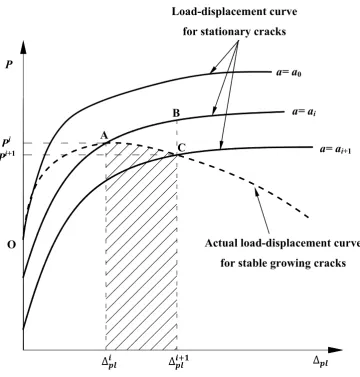
load versus LLD curve. Figure 2.3 shows a typical load vs. displacement curve in the fracture toughness test. The total area under the loading path, A, is defined as the work done by external force during the test. As indicated in Fig. 2.3, A can be separated by an elastic unloading path into an elastic component, Ael, and a plastic component, Apl, i.e. A

= Ael+ Apl. Similarly, this unloading path separates Δ into an elastic component, Δel, and

a plastic component, Δpl, i.e. Δ = Δel+ Δpl, and Eq. (2.3) can be accordingly rewritten as

0 0

1 el 1 pl

el pl el pl

P P

J d d J J

B a B a

   

      

 



(2.5)

where Jel and Jpl are the elastic and plastic components of J, respectively. Jel can be

determined from the stress intensity factor K (Anderson, 2005):

2₍₁ 2₎

el K J E    (2.6)

where E and v are Young’s modulus and Poisson’s ratio respectively. Sumpter and Turner (1976) proposed the following equation to compute Jpl:

0

LLD LLD

pl

LLD

pl pl pl

pl pl

A

J Pd

bB bB

  





  (2.7)

where and denote the plastic geometry factor and plastic area under the load versus load line displacement respectively. Alternatively, J can be evaluated from the crack mouth opening displacement (CMOD or V) as opposed to LLD (Kirk and Dodds, 1993); therefore,

0

 CMOD



pl  CMOD

CMOD V

pl pl pl

(34)

where represents the plastic area under the load versus CMOD curve, and denotes the CMOD-based plastic geometry factor.

Equations (2.1) through (2.8) are limited to stationary cracks. The crack growth correction should be considered in the evaluation of J for growing cracks. Based on the deformation theory of plasticity, J is independent of the load path leading to the current

LLD (or CMOD) and crack length a, given that the J-controlled crack growth conditions are satisfied (Sumpter and Turner, 1976). Accordingly, J is a function of two independent variables, a and Δ. Ernst et al. (1981) developed an incremental method to estimate J for growing cracks by deriving the total differential of Jpl as

 pl  

pl pl pl

P

dJ d J da

bB b





(2.9) with 1 1 ( / )    _   _ _   pl pl pl b

W a W

  

 (2.10)

Integrating both sides of Eq. (2.9) yields

0





_

pl _pl  

_

a

pl pl _a pl

P

J d J da

bB b





(2.11)

where a0 is the initial crack length. Equation (2.11) can be applied to any loading path leading to the current values of Δpl and a. Figure 2.4 shows a schematic of the estimation of Jpl for growing cracks. The figure includes a typical P-Δpl curve for a growing crack,

(35)

, 1

 

i pl

B i i i

pl pl pl

i

J J A

b B



(2.12)

where is the value of Jpl at A or step i; is the value of Jpl at B or the intermediate

value of Jpl between step i and step i+1; bi = W - ai, and , equals the area of

ABΔ Δ but can be adequately approximated by the area under the actual loading path between Δ and Δ (i.e. the shaded area in Fig. 2.4), if ∆ ∆ is sufficiently small;

, _{can be evaluated using the trapezoidal rule as} , _≅ _∆ _∆ _.

Integrating both sides of Eq. (2.9) again along the loading path BC results in





1 1 1      _   _  

i B i

pl pl i i

i

J J a a

b



(2.13)

where is the value of Jpl at C or step i+1. Combining Eqs. (2.12) and (2.13) leads to

the following general incremental expression for calculating Jpl:





1 , 1

1 1        _  _{ }   _     i pl

i i i i i

pl pl pl i i

i i

J J A a a

b B b

 

(2.14)

Equation (2.14) is adopted by ASTM E1820-11E2 (ASTM, 2013) as the main procedure to experimentally evaluate the J-R curve. The crack length corresponding to each loading step can be determined using the unloading compliance method, which is described in Appendix B. Parameters ηpl and γ are called plastic geometry factors serving as key

parameters to the experimental evaluation of the J-integral. The evaluation of the ηpl

(36)

2.1.3 Literature Review of Studies on the Plastic Geometry Factors

Early studies (Begley and Landes, 1972; Rice et al., 1973) showed that the J-integral, interpreted as a nonlinear energy release rate, is related to the area under the P-LLD curve. The total J-integral can be separated into the elastic component Jel and the plastic

component Jpl. It is straightforward to evaluate Jel based on the linear elastic stress

intensity factor, the solution of which is well documented (e.g. Tada et al., 2000). Sumpter and Turner (1976) proposed the dimensionless plastic η factor (ηpl) to evaluate Jpl by relating Jpl to the plastic work that can be computed from the P-LLD or P-CMOD

curve. At the limit load, the η factor is only a function of the configuration of the cracked body and independent of the loading (Kanninen and Popelar, 1985).

Due to its simplicity, the ηpl–based evaluation of J-integral is widely used and adopted in

standards such as ASTM E1820-11E2 and BS7448-97. It follows that accurate ηpl factors

are needed to ensure the accuracy of the experimentally-evaluated J. Wu et al. (1990) applied the slip line field solution to derive the analytic solution of ηpl factors.

Sharobeam and Landes (1991) adopted the load separation analysis proposed by Paris et al. (1980) to develop an experimental procedure to determine ηpl factors. Based on the

two-dimensional (2D) plane-strain finite element analysis (FEA), both LLD- and CMOD -based ηpl have been developed for the standard deeply-cracked (i.e. the relative crack

length a/W greater than or equal to 0.45) SE(B) and C(T) specimen. For example, Kirk and Dodds (1993) and Donato and Ruggieri (2006) carried out 2D plane-strain FEA on SE(B) specimens to evaluate both LLD- and CMOD-based ηpl whereas the estimation of LLD- and CMOD-based ηpl for C(T) specimens was included in the study by Kim and

Schwalbe (2001). The LLD-based ηpl is reported (Wu et al., 1990; Kim and Schwalbe,

2001) to be independent of a/W for deeply-cracked SE(B) and C(T), and the CMOD -based ηpl is found to be less dependent on the strain hardening exponent n than LLD

-based ηpl for shallow-cracked SE(B) (Kirk and Dodds, 1993; Kim and Schwalbe, 2001;

(37)

It is well known that the J-R curve is dependent on the crack tip constraint (Yuan and Brocks, 1998). Recent studies on ηpl (e.g. Shen and Tyson, 2009; Petti et al., 2009) have

focused on non-standard specimens with low levels of constraint including the single-edge tension (SE(T)) and shallow-cracked SE(B) specimens. Both LLD- and CMOD -based ηpl are observed to be a function of a/W for shallow-cracked SE(B) and SE(T)

specimens (Kirk and Dodds, 1993; Link and Joyce, 1995; Cravero and Ruggieri, 2007).

With the rapid advancement of modern computers, three-dimensional (3D) FEA are being increasingly used to evaluate ηpl. Nevalainen and Dodds (1995) obtained values of

ηpl for the SE(B) and C(T) specimens based on 3D FEA. Kim et al. (2004) evaluated ηpl

for plane-sided SE(B), SE(T) and C(T) specimen using 3D FEA. In these studies, ηpl

corresponding to both the average and maximum J values over the crack front, i.e. ηave

and ηmax, were evaluated. In the study by Nikishkov et al. (1999), 3D SE(B) and C(T)

specimens with curved crack fronts were analyzed to evaluate ηpl corresponding to the

local J value at the mid-thickness of the crack front, ηmid. Work done by Kulka and

Sherry (2012) was focused on the LLD-based ηavefor C(T) specimens with various a/W

ratios and thickness-to-width (B/W) ratios. In the study by Ruggieri (2012), 3D FEA was carried out to evaluate ηplfor plane-sided SE(T) specimens with a wide range of a/W

ratios (0.3 to 0.7) and two different specimens thicknesses. The η factors for side-grooved SE(B) and C(T) models with specific a/W ratios and B/W ratios have also been reported in the literature (Nikishkov et al., 1999; Nevalainen and Dodds, 1995).

2.1.4 Objective and Approach

Several observations of the previous studies on ηpl are in order. First, ηpl determined from

2D FEA may not be adequate given that the real specimens and cracks are three-dimensional. Second, although ηpl determined from 3D FEA has been reported in the

literature, there is a lack of systematic investigations of ηpl that take into account the

impact of a/W, B/W, side-grooves and strain hardening characteristics on ηpl. Finally, all

(38)

front (Dodds et al., 1990). For shallow-cracked specimens where the crack tip is near the crack month at which CMOD is measured, it is expected that using the large-strain analysis may lead to more accurate simulation and values of ηpl. To the best knowledge

of the author of this thesis, the use of the large-strain 3D FEA to evaluate ηpl has not been

explored in the literature.

Motivated by these observations, a systematic investigation of ηpl for SE(B) specimens

using the large-displacement large-strain 3D FEA was carried out in this study. Both plane-sided and side-grooved SE(B) specimens with a wide range of a/W and B/W ratios were analyzed. The LLD- and CMOD-based ηpl corresponding to the average J value

over the crack front as well as the local J at the mid-plane were evaluated. The impact of

a/W, B/W and the strain hardening characteristics on the η factor was also investigated. The research outcome will improve the accuracy of the J-R curve obtained from the experiment and facilitate the evaluation of J-R curves using non-standard (e.g. shallow-cracked) SE(B) specimens.

The organization of this chapter is as follows. Section 2.2 describes the finite element analysis involved in the present study. The evaluation procedure of plastic η factor is presented in Section 2.3, accompanied by the analysis results and comparison with those reported in the literature. The conclusions of this chapter are summarized in Section 2.4.

2.2 Finite

Element Analysis

2.2.1 Material Model

Evaluation of ηpl requires computation of J and the load-displacement response involving

(39)

(Mase, 1970). The use of the small-displacement formulation basically ignores the difference between the spatial and material coordinate systems, whereas the large-displacement formulation takes this difference into account and the Lagrangian coordinate system was selected in this study (ADINA, 2012). In ADINA, the large-displacement large-strain formulation requires input of the Cauchy (true) stress-logarithmic (true) strain and outputs the Cauchy stress and deformation gradient. The von Mises yield criterion and isotropic hardening rule were adopted in the analysis. The von Mises yield criterion states that yielding starts once the second invariant of the deviatoric stress tensor, J2, reaches a critical value (i.e. σy2/3). The incremental theory of

plasticity combined with the associate flow rule and von Mises yield criterion can be characterized by the following constitutive equation:

pl

ij ij

d ds (2.15)

where and sij are the plastic strain tensor and the deviatoric stress tensor, respectively,

and dλ is a scalar factor of proportionality.

The Ramberg-Osgood stress-strain relationship as given by Eq. (1.7) was employed. In this study, materials with σ0 = 550 MPa, E = 200 GPa, ν = 0.3 and  = 1 were selected to simulate the X80 (API, 2012) grade pipeline steel. Three values of the strain hardening exponent, namely n= 5, 10 and 15, were considered to investigate the effect of n on ηpl.

Note that the cases with n = 10 were considered as the baseline cases, as n = 10 is representative of the strain hardening characteristics of the X80 pipeline steels.

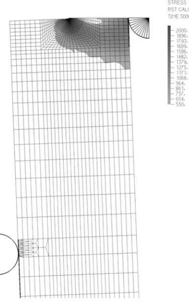
2.2.2 Finite Element Model

The geometric configuration of a typical SE(B) specimen in the FEA is shown in Fig. 2.5 together with the fixation and loading conditions. All the specimens included in this study have a width (W) of 20 mm and a span (S) of 4W. For the baseline cases (i.e. n =

(40)

considered. Both plane-sided (PS) and side-grooved (SG) specimens were modeled. For the latter, the side groove was modeled as a sharp V-notch of 45 degrees with a depth of 10%B on each side of the specimen, which is consistent with the recommendations in ASTM E1820-11E2 (ASTM, 2013). A side-grooved model with a/W = 0.5 and B/W = 0.5 is schematically shown in Fig. 2.6. For the sensitivity cases with n = 15, only plane-sided specimens with three crack lengths (i.e. a/W = 0.3, 0.5 and 0.7) and B/W = 0.5 were investigated. Due to symmetry, only a quarter of a given specimen was modeled in the FEA. The 8-node 3D brick elements with 2×2×2 integration were used; the accuracy of using such element to calculate J for SE(B) specimens has been shown to be adequate (Kulka and Sherry, 2012).

A blunt crack tip with a radius rw = 0.003 mm (see Fig. 2.5) was modeled to facilitate the

large-deformation calculation (Graba, 2007). Note that for the side-grooved specimens, the blunt crack tip is also prepared through the thickness of the side grooves as shown in Fig. 2.6 to mitigate the impact of the singularity caused by the sharp V-notch under tension on the finite strain analysis. A spider-web mesh around the crack tip was established with 40 concentric semicircles (i.e. rings) surrounding the crack tip. The in-plane size of the elements closest to the crack tip is around 0.003 mm, and about 1/100 of the in-plane size of the elements in the outermost ring. The aspect ratio of these elements is set to be less than 10. The model was divided into 8 and 15 layers along the thickness direction for PS and SG specimens, respectively. The mesh density increases from the mid plane to the free surface to capture the high stress gradients near the free surface. A sensitivity study of the meshing was carried out, and the results indicated that further increasing the number of layers along the thickness has little impact on the calculation of both the local J value at the midpoint of the crack front, Jmid, and the average J value over

the entire crack front, Jave. The total number of elements is approximately 15,000 in a

(41)

2.2.3 Computational Procedure

Displacement-controlled loading was applied in all the models. For models with a/W ≥

0.4, the displacement was increased from 0 to 1.5 mm through 5000 steps, whereas it was increased from 0 to 2 ~ 2.5 mm through 15,000 steps for models with a/W = 0.3. The sparse matrix solver was selected for its high efficiency in numerical analysis (ADINA, 2012). The full Newton-Raphson iteration method was adopted to find the solution of nonlinear equations with the maximum number of iterations for each step being 50. The displacement convergence criterion was selected, in which the displacement tolerance equaled 0.0001 corresponding to a reference displacement of 1 mm (ADINA, 2012). Figure 2.7 shows the distribution of the effective stress in a typical specimen (i.e. a/W = 0.5 and B/W = 1) corresponding to the applied displacement of 1.5mm. The shaded area denotes the extent of the plastic zone where the effective stress is greater than or equal to the yield strength (i.e. 550 MPa). The magnitude of the total strain in the element around the crack tip is about 1 - 10%. The J-integral was computed by using the virtual crack extension method implemented in ADINA (Anderson, 2005; ADINA, 2012). A brief description of this method is included in Appendix A. To ensure the path-independence of the calculated J values, the two outermost semicircular rings surrounding the crack tip were used to define the virtual shifts. Both Jmid and Jave were calculated and used to

evaluate the corresponding ηpl factors. By subtracting the elastic component of J from

the total J as described in Eqs. (2.5) and (2.6), the plastic component of J, Jpl, can be

(42)

2.3 Determination of Plastic Geometry Factors for SE(B)

Specimens

2.3.1 Evaluation Procedure of Plastic Geometry Factors

The ηpl factors can be computed at a given loading level (i.e. J value) using the following

expression (Ruggieri, 2012):

0 2 0                pl

pl N pl

pl

pl pl

N J

J bB b J

A A A b B    (2.16)

where BN denotes the net thickness of the specimen, i.e. BN = B for the plane-sided

specimen and BN = 0.8B for the side-grooved specimen with the side-groove depth equal

to 0.1B at each side, and ̅ and ̅ are non-dimensionalized J and plastic area, respectively. Depending on the load-displacement curve (i.e. the P-LLD or P-CMOD

curve) and Jpl value (i.e. Jpl evaluated from Jmid or Jave) used in Eq. (2.16), four different

ηpl factors can be evaluated, namely , , and , where the subscript

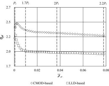
“pl” is omitted to reduce clutter. Figure 2.8 shows the variation of ηpl with ̅ for a

representative specimen (plane-sided, a/W = 0.7, B/W = 1 and n = 10). The figure suggests that ηpl is load-dependent for P ≤ 1.7Pl, where Pl is the reference load and

defined as BNb2σ0/S (Nevalainen and Dodds, 1995), and becomes approximately independent of the load for P > 1.7Pl. Figures 2.9(a) and 2.9(b) depict the relationships

between ̅ and CMOD-based ̅ as well as between ̅ and LLD-based ̅ for four specimens (two plane-sided and two side-grooved) with a/W = 0.3 and 0.7 and n = 10. The ηpl factor can be evaluated as the slope of the linear fit of ̅ vs. ̅ . Note that in a

number of previous studies, ηpl for SE(B) specimens was evaluated by fitting the ̅ vs.

̅ data corresponding to high levels of applied load. For example, Kirk and Dodds

(43)

̅ ≤ 0.25 (approximately equivalent to 1.1Pl ≤P≤ 2.5Pl); Petti et al. (2009) evaluated

ηpl by fitting data starting from bσ0/Jave = 50 (approximately equivalent to P≥ 1.6Pl). As

such, evaluating ηpl at high loading levels minimizes the load-dependency of ηpl as

indicated in Fig. 2.8.

In the present study, it is found that the range of the data used in the fitting has a non-negligible impact on the value of ηpl. For instance, ηpl determined based on data within

the range of 1.0Pl≤P≤ 1.7Pl is approximately 10% larger then that based on data within

the range of 1.0Pl≤P≤ 2.0Pl for deeply cracked (e.g. a/W = 0.7) specimens with n = 5.

The J-R curve tests involving SE(B) specimens carried out in a previous study (Wang et al., 2012) indicate that the maximum loading level is typically less than 2.2Pl for

materials with n = 10. On the other hand, because of the use of the large-strain formulation, the J value for shallow cracked specimens calculated in the present study was observed to be path-dependent once the loading level exceeds 1.7Pl.

Based on these considerations, in this study, the ηpl factors for specimens with a/W≥ 0.4

were evaluated by linearly fitting the ̅ vs. ̅ data corresponding to 1.0Pl ≤P≤ 2.0Pl.

The ηpl factors for specimens with a/W = 0.3 were evaluated based on data within the

range of 1.0Pl ≤P≤ 1.7Pl.

2.3.2 Results and Discussions

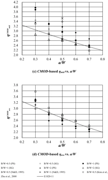
Both CMOD- and LLD-based ηpl values corresponding to n = 10 are calculated and listed

in Table 2.1. Figure 2.10 shows the calculated CMOD- and LLD-based ηpl values plotted

against a/W for both PS and SG specimens with n = 10 and different B/W ratios. Figures. 2.10a and 2.10b indicate that the LLD-based ηpl generally increases with the a/W ratio,

(44)

B/W ratios is approximately 9.5%. The values of and for the SG models are generally 2-25% lower than those for the PS models with the same a/W, B/W and n

values, whereas and for the SG models are 1-6% higher than those for the corresponding PS models.

The ηpl values obtained in this study are compared with those reported by Nevalainen and

Dodds (1995) (N&D, 1995) and Kim et al. (2004) in Fig. 2.10, which are obtained from 3D FEA using the small-strain formulation. Both studies are focused on the PS models; therefore, only the ηpl values corresponding to their PS models are shown for comparison.

The ηpl values obtained in this study are generally lower than those reported by Kim et al.

and Nevalainen and Dodds with the relative difference ranging from 4% to 11%. These differences may be due to the fact that the ηpl values obtained in this study are based on

the large strain formulation adopted in the FEA.

Zhu et al. (2008) proposed the following expressions of LLD- and CMOD-based ηplfor

SE(B) specimensby fitting the results from both 2D plane strain (PE) and 3D FEA with the small-strain formulation reported in the literature:









2

1.620 0.850 / 0.651 / , 0.25 / 0.7

LLD

pl a W a W a W

       (2.17)









2

3.667 2.199 / 0.437 / , 0.05 / 0.7

     

CMOD

pl a W a W a W

 (2.18)

It is worth pointing out that Eq. (2.18) has been adopted by ASTM E1820-11E2 (ASTM, 2013) for CMOD-based evaluation of J in the J-R curve test. As for LLD-based evaluation of J, ASTM E1820-11E2 suggests = 1.9 for deeply cracked (i.e. 0.45≤

Finite Element Analyses of Single-Edge Bend Specimens for J-R Curve Development

Scholarship@Western

Scholarship@Western

Finite Element Analyses of Single-Edge Bend Specimens for J-R

Finite Element Analyses of Single-Edge Bend Specimens for J-R

Curve Development

Curve Development

Abstract

Keywords

Co-Authorship

Dedication

Acknowledgments

Table of Contents

List of Tables

List of Figures

List of Nomenclature

Chapter 1 Introduction

1.1 Background

1.2 Fundamentals of Fracture Mechanics

1.2.1 Linear Elastic Fracture Mechanics

 

 

 

1.2.2 Elastic Plastic Fracture Mechanics



 

 



 

1.3 Objective and Research Significance

1.3.1 Investigation of Plastic Geometry Factors

1.3.2 Investigation of Constraint-corrected

J

-

R

Curve

1.4 Thesis

Outline

References

Chapter 2 Evaluation of Plastic

η

Factors for SE(B)

Specimens Based on Three-dimensional Finite Element

Analysis

2.1 Background

and

Objective

2.1.1

J

-

R

Curve on Small-scale Specimens

2.1.2 Estimation of

J

Using Plastic Geometry Factors

































2.1.3 Literature Review of Studies on the Plastic Geometry Factors

2.1.4 Objective and Approach

2.2 Finite

Element Analysis

2.2.1 Material Model

2.2.2 Finite Element Model

2.2.3 Computational Procedure

2.3 Determination of Plastic Geometry Factors for SE(B)

Specimens

_

_

_