Phase object pattern recognition by optical correlation using a liquid crystal display for spatial phase modulation

(1)

Phase Object Pattern Recognition

by Optical Correlation

using a Liquid Crystal Display

for Spatial Phase Modulation

Mark Charles Gardner

December 2002

University College London

UCL

(2)

ProQuest Number: U644152

INFORMATION TO ALL USERS

The quality of this reproduction is dependent upon the quality of the copy submitted. In the unlikely event that the author did not send a complete manuscript and there are missing pages, these will be noted. Also, if material had to be removed,

a note will indicate the deletion.

uest.

ProQuest U644152

This work is protected against unauthorized copying under Title 17, United States Code. Microform Edition © ProQuest LLC.

ProQuest LLC

789 East Eisenhower Parkway P.O. Box 1346

(3)

ACKNOWLEDGEMENTS

First and foremost I must thank my primary supervisor, Sally Day at UCL, for her

patient support and guidance. David Selviah is thanked for a great deal of advice and

enthusiasm for the project. I am grateful to Robert Renton for continuing the high

standard o f secondary supervision at Sira following the departure of Greg Gregoriou

after ten months. Thanks to John Gilby at Sira who's experience and knowledge of

machine imaging proved most useful.

A special thanks is due to the other students working on Liquid Crystal Display

projects: Robin Kilpatrick and Sue Blakeney and for the co-operative atmosphere that

developed. In addition is was a pleasure working with all the students sharing the

UCL office throughout the period of the research: Chi-Ching Chang, Lawrence

Commander, Keith Forward, Teriyuki, Kataoka, Laki Panteli, Notis Stamos and Tim

York and all the others in the Optical Systems and Devices group. I would like to

acknowledge the department of electrical engineering’s clean room staff: Kevin Lee

and Vic Law for their helpfulness whenever I needed to use their facilities.

The project was sponsored by Philips Research Laboratories who kindly provided the

Liquid Crystal Display. Thanks especially to Andy Pearson, David Parker and Alan

Knapp for their assistance and provision of data concerning the LCD.

A number of staff at Sira deserve special thanks for their help. Tom Williams (for all

manner of optics advice), Neil Kinnear (who could knock up an enclosure or

mounting plate to the highest standard using the minimum of specifications), Mark

Hodgetts, Neil Stewart, James Dean (always willing to sort out a computer at short

notice) and Tony Alnut. Non-technical support staff who's help made life easier

include Linda Huntingford (the fabric canopy of the light exclusion tent was due to

her handiwork), her successor Malanie Holmes and Dianne MacGraw.

The work was supported by the Engineering and Physical Sciences Research Council

(4)

ABSTRACT

Optical correlation is demonstrated as a means of automatic inspection of 3D objects

with depth features in the order of a wavelength of light. The distorted wave-front

from the object is directly subjected to pattern recognition. Thus, use is made of the

full complex light field from the object. Normally in optical correlation the phase part,

and hence any useful information associated with it, is discarded through electronic

capture and redisplay o f the object.

A commercial Liquid Crystal Display (LCD) is utilised as an optical Fourier plane

filter medium, affording the high spatial resolution of 'purpose made' spatial light

modulators (SLMs), but at lower cost and with simple drive signal requirements.

While LCDs are designed as intensity modulators, it is known that in the spatial

frequency domain, phase manipulation is more effective than intensity manipulation.

The LCD's polariser and analyzer orientation is engineered to provide up to 229° of

phase modulation (despite an LC layer thickness of less than 4.5}im) with insignificant

coupled intensity modulation. A model developed in the UCL/Sira research group to

show complex modulation as a function of polariser / analyzer configuration is

experimentally evaluated. An improvement to the model showing the importance of

including effective LC cell capacitance is also detailed. The LCD system's response to

high spatial frequency images is investigated, and an algorithm, devised to process

images prior to display, is described. While proving useful for visual display

purposes, it was not found suitable for correlation filter display.

A complete correlator is designed and constructed to accommodate small holographic

optical elements at the input. The correlator is shown to discriminate successfully

between real (not displayed) transparent objects, with 3D relief patterning for, it is

believed, the first time. Experiments show good agreement with computer

simulations despite the poor display of high spatial frequencies in the filter plane.

While identically patterned input objects of varying depth yield sluggish

discrimination, simulations were run which suggested adequate depth discrimination

would be achievable using full complex Fourier plane filtering. Finally an automatic

(5)

LIST OF

ABBREVIATIONS AND SYMBOLS

AMLCD active matrix liquid crystal display

AGF amplitude only filter

BPOF binary phase only filter

CMF complex matched filter

F Fourier Transform operator

FFT fast Fourier transform

FT Fourier transform

FLC ferroelectric liquid crystal

FTL Fourier transform lens

FZP Fresnel zone plate

GL grey level

HOE holographic optical element

ITO indium tin oxide

IGF intensity only filter

j square root o f- 1

JTC joint transform correlator

JTPS joint transform power spectrum

k wave-number

LC liquid crystal (the material)

LCD liquid crystal display (the device)

LCLV liquid crystal light valve

MZ Mach-Zehnder (interferometer)

«e extraordinary refractive index in a biréfringent material

rio ordinary refractive index in a biréfringent material

«X effective refractive index in a biréfringent material for an arbitrary

angle of incidence

NDF neutral density filter

GA optic axis (of a biréfringent component)

GASLM optically addressed SLM

GFT optical Fourier transform

PMC phase modulation capability

PGF phase only filter

QWP quarter wave plate

5 spatial frequency : kllK (cycles per metre)

SDF synthetic discriminant function

SFD self focusing Dammann grating

SLM spatial light modulator

TFD thin film diode

TFT thin film transistor

TNLCD twisted nematic liquid crystal display

VGA video graphics adapter (computer display convention)

(6)

P birefringence parameter

iSn optical anisotropy ; n^- Uo

^,T| horizontal and vertical axes in the spatial frequency domain

corresponding to x,y in the spatial domain

(8> convolution operator

o cross-correlation operator

X* complex conjugate of x

4-f correlator architecture type measuring four focal lengths with a

central filter plane

NOTE:

Fourier transformation is sometimes indicated by capitalization of the signal being

transformed with the reciprocal dimension as the variable.

i.e. % ) = "Fourier transform of function; 5(jc)" = F [5(x)]

Notation for the impulse response and transfer function are similarly constructed:

i.e.

h(t) is the impulse response (temporal domain),

(7)

no

111 112 113 114 115 117 118 120 120 121 122 123 CHAPTER 6

EXAMINATION OF LCD MODULATION UNDER HIGH SPATIAL FREQUENCY CONDITIONS

6.1 INTRODUCTION ...

6.2 EXAMINING TRANSMISSION THROUGH A SINGLE LCD PIXEL

6.2.1 I n i t i a l m e a s u r e m e n t o f t r a n s m i s s i o n a s a f u n c t i o n o f c o lu m n p o s i t io n

6.3 PLOTTING THE NEIGHBOURING COLUMN INFLUENCE ...

6.3.1 D e t a i l e d MEASUREMENTS ...

6.3.2 A CONVOLUTION DESCRIPTION OF NEIGHBOURING COLUMN INFLUENCE

6.3 .2.1 Kernel change with column position type

6.3.2.2 Restricted dynamic range ...

6.3.2.3 Kernel weight emphasis ...

6.3.3 E x p e r i m e n t a l m e a s u r e m e n t o f d e c o n v o l u t i o n p r o g r a m e f f i c a c y ...

6.3.3 .1 Unprocessed test image display

6.3.3.2 Deconvolved test image display

6.4 COMPARISON OF DECONVOLUTION METHOD WITH AN ITERATIVE

OPTIMISATION METHOD ...

6.5 A PICTORIAL DEMONSTRATION OF THE DECONVOLUTION ALGORITHM

6.6 SUMMARY OF DEALING WITH ADJACENT COLUMN INFLUENCE

(10)

C H A P T E R 7 147

O P T I C A L C O R R E L A T I O N O F P H A S E O B J E C T S

7.1 IN T R O D U C T IO N 147

1 2 IN T E N S IT Y M A T C H E D F IL T E R F O R A PE R T U R E O B JE C T S ... 148

7 .2 .1 O F T BASED In t e n s it y On l y Filter ... ... ... ... 148

7 .2 .1 .1 O F T o r ig in lo c a tio n ... ... ... ... ... 149

7 .2 .1 .2 O F T r e siz in g ... ... ... ... ... ... 149

7 .2 .1 .3 B ack grou n d r em o v a l and in ten sity sc a lin g ... ... ... 149

7 .2 .1 .4 D isp la y in g th e filte r ... ... ... ... ... 150

7 .2 .2 O F T In t e n s it y CORRELATION RESULTS ... ... ... ... 150

7 .2 .3 FFT BASED In t e n s it y On l y Filt er ... ... ... ... 151

7 .2 .3 .1 F FT com p u tation ... ... ... ... ... 151

7 .2 .3 .2 2 D FFT r e siz in g fo r L C D p resen tation ... ... ... 152

7 .3 P H A S E O N L Y FILTER S 153

7 .3 .1 Bin a r y Ph a se On l y Fil t e r (B P O F ) ... ... ... ... 153

7 .3 .2 2 5 6 -le v e l Ph a se On l y Fil t e r ... ... ... ... ... 154

7 .4 C O R R E L A T IO N O F P H A S E O B JE C T S ... 157

7 .4 .1 PO F CONSTRUCTION FOR Ph a s e Ob je c t s ... ... ... ... 160

7 .4 .2 Ou t p u ta n a l y s ism e t h o df o r Ph a se Obje c tc o r r e l a t io ne x p e r im e n t s 162

7 .4 .3 Au t o-c o r r e l a t io n OF Ph a s e Obje c t s ... ... ... ... 162

CHAPTER 8 165

PHASE OBJECT CROSS CORRELATION AND FACTORS AFFECTING RECOGNITION

8.1 PHASE OBJECT CROSS-CORRELATION 165

8 .1 .1 S im u la t i o n o f C r o s s - c o r r e l a t i o n w i t h D i f f e r e n t P a t t e r n s a n d

SIMILAR DEPTHS ... ... ... ... ... ... ... 165

8 .1 .2 S i m u la t i o n o f C r o s s - c o r r e l a t i o n w i t h S im ila r P a t t e r n s a n d

D i f f e r e n t D e p t h s ... ... ... ... ... ... 166

8 .1 .3 E x p e r im e n t a l P h a s e O b j e c t C r o s s - c o r r e l a t i o n w i t h D i f f e r e n t

P a t t e r n s AND S im ila r D e p t h s ... ... ... ... ... 168

8 .1 .4 E x p e r im e n t a l P h a s e O b j e c t C r o s s - c o r r e l a t i o n w i t h S im il a r P a t t e r n s

AND D i f f e r e n t DEPTHS ... ... ... ... ... ... 170

8 .1 .5 P h a s e OBJECT CROSS CORRELATION REMARKS ... ... ... 173

8 .2 AUTO-CORRELATION SENSITIVITY TO OBJECT Z -P O S IT IO N ... 173

8.3 AUTO-CORRELATION SENSITIVITY TO FILTER QUANTIZATION ... 174

8 .4 PHASE OBJECT CORRELATION IN INTENSITY N O I S E ... 178

CHAPTER 9

DISCUSSION AND CONCLUSIONS

9.1 INTRODUCTION TO CONCLUSIONS AND DISCUSSION

9.2 BRIEF SUMMARY OF MAIN A C H IEV EM EN TS...

9.2.1 A p p lic a t io n o f a c o r r e l a t o r u s i n g a c o m m e r c i a l LCD t o r e a l

PHASE OBJECTS ...

9.2.2 C o r r e l a t o r d e s i g n a n d c o n s t r u c t i o n - s tr a n d (i)

9.2.3 LCD MODULATION CHARACTERISTICS - STRAND (ll)

9.3 DETAILS OF THE FINDINGS ...

9.3.1 C o r r e l a t o r CONSTRUCTION

9.3.2 LCD U n if o r m M o d u l a t i o n

9.3.3 LCD H ig h S p a t i a l F r e q u e n c y M o d u l a t i o n

9.3.4 A u t o - c o r r e l a t i o n

9.3.5 C r o s s - c o r r e l a t i o n

(11)

9 .3 .7 Mu l tipl ic a t iv e INTENSITY NOISE

9 .3 .8 Ob j e c t'z'POSITION

9 .4 COLLATION AND DISCUSSION OF F IN D IN G S ...

9 .5 FUTURE WORK ...

9 .5 .1 Theeffecto f Te m p o r a l Fl u c t u a t io n sin Filters

9 .5 .2 Ex p l o it in gc o u p l e dm o d u l a t io nfo r Depth Disc r im in a t io n

9 .5 .3 Ou t-o f-Pl a n e INPUT OBJECTS

9 .5 .4 Bio l o g ic a lr e c o g n it io nu s in g Dist o r t io n In v a r ia n c e

9 .6 CLOSING REMARKS ...

188 189 189 192 192 192 192 193 193 APPENDIX A

OPTICAL FOURIER TRANSFORMATION & CORRELATION

A. 1 INTRODUCTION TO APPENDIX A ...

A .I.l T h e F o u r ie r TRANSFORM

A. 1.2 T h e C o n v o l u t i o n F u n c t i o n

A. 1.3 T h e C r o s s - C o r r e l a t i o n F u n c t i o n

A. 2 OPTICAL DIFFRACTION - THE MEANS TO OPTICAL CORRELATION

A.2.1 B a c k g r o u n d

A.2.2 T h e F r e s n e l APPROXIMATIONS

A.2.3 T h e F r a u n h o f e r APPROXIMATIONS...

A.2.4 S p a t i a l FILTERING

195 195 195 195 197 198 198 199 202 203 APPENDIX B

JONES CALCULUS 205

APPENDIX C

MATLAB LISTING FOR DECONVOLUTION BASED PROCESSING 207

APPENDIX D

MATLAB LISTING FOR OPTICAL CORRELATION 210

(12)

LIST OF FIGURES

CHAPTER 2

2.1 The effect of a processing element, A, on a signal,/

(a) in the time domain, (b) in the frequency domain. ... ... ... ... 23

2.2 Co-ordinate system used for the Fresnel approximation. ... ... ... 26

2.3 Schematic diagram of a 4-f Spatial Filter. ... ... ... ... ... 28

2.4 Method for recording a Vander Lugt complex filter. ... ... ... ... 29

2.5 Demoli's coherent averaging scheme to produce a filter based on a set of

in-class examples. ... ... ... ... ... ... ... 40

CHAPTER 3

3.1 Molecular arrangement of Nematic Liquid Crystal. ... ... ... ... 50

3.2 Molecular arrangement of Chiral Nematic Liquid Crystal. ... ... ... 51

3.3 Molecular arrangement in; (a) Smectic A liquid crystal, (b) Smectic C liquid crystal. 52

3.4 The three deformation types; (a) Splay, (b) Twist, (c) Bend. ... ... ... 53

3.5 Structure of TN liquid crystal cell showing director orientation for a clockwise twist

direction (not to scale). ... ... ... ... ... ... ... 55

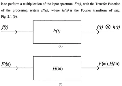
3.6 Index Ellipsoid representation of effective refractive index. ... ... ... 57

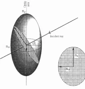
3.7 Typical transmission vs. voltage curve for TNLCD between crossed polarisers showing

how the sum of row and column voltages in a passive matrix display provides access to the near linear part of the characteristic while applying a row voltage alone barely clears

the optical threshold. ... ... ... ... ... ... ... 58

3.8 Illustration of the bi-stable behaviour of an FLC device where a small gap between

substrates inhibits the director rotation between adjacent Smectic C planes. ... 60

3.9 Accommodation of bi-stable states of director orientation in chevron structure. ... 61

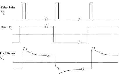
3.10 Passive matrix pixel construction. ... ... ... ... ... ... 63

3.11 Timing diagram illustrating passive matrix addressing. ... ... ... 63

3.12 Typical transmission vs voltage curve for TNLCD between crossed polarisers

showing that in passive matrix addressing the intensity dynamic range depends on the

ratio of Vqnto Vq f f• • • • ■ • • • ■ • • • • • • • • • • • 64

3.13 Typical TFT connection scheme. Cp is the I.e. pixel electrode capacitance. ... 65

3 .14 TFT waveforms showing voltage step due to coupling of reset pulse through parasitic

capacitance, Cqd ■ ... ... ... ... ... ... ... 67

3.15 TFD connection schemes; a) bi-directional, b) ring, c) back-to-back. ... ... 68

3.16 OASLM construction. ... ... ... ... ... ... ... 69

3.17 Representation of a Rotated Eigenvector. ... ... ... ... ... 78

3.18 Calculated phase, 5, for the two eigenvectors of a 90° TN cell. (Based on ref. Dav98). 79

3.19 Calculated ellipticity of Rotated Eigenvectors of a 90° TN cell. (Based on ref. Dav98). 79

CHAPTER 4

4.1 Procedure for Fourier Transform Lens selection and its impact on correlator

performance. ... ... ... ... ... ... ... ... 87

4.2 Using a known grating to measure the true focal length of the Fourier Transform Lens

using a grating of known frequency. ... ... ... ... ... 89

4.3 Spacing of diffracted images at the output plane. ... ... ... ... 90

4.4 Highest spatial frequency admitted by the filter. ... ... ... ... 90

4.5 Spatial filter and beam expander. The collimator lens to object distance may be less

than the lens focal length, reducing the overall length of the correlator. ... 93

4.6 Correlator component layout, showing the important dimensions in mm. ... 94

4.7 Measured output image grey level as a function on incident intensity. ... ... 97

4.8 Interconnection of hardware making up the correlator system.... ... ... 98

CHAPTER 5

5.1 Layout of optical components for intensity transmission measurement. ... ... 101

5.2 Effects of the Brightness and Contrast controls on LCD intensity transmission between

crossed polarizers. Examples are shown illustrating the accessible region of the

(13)

5.3 Intensity transmission as a function of brightness for maximum and minimum grey

level (contrast set to minimum). ... ... ... ... ... ... 103

5.4 Determination of grey level to voltage relationship for maximum contrast, minimum

Brightness settings;

a) Measured intensity transmission against applied grey level for LDK036T-20 LCD between +/- 45° polarizers. (The 100% value is that with no power supplied to the device). b) Measured intensity transmission against applied voltage (rms) for the Test Cell between +/- 45° polarizers

c) Cross reference between grey level and voltage. ... ... ... ... 105

5.5 Modelled and measured intensity transmission for the LDK036T-20 LCD between

+/-45° polarizers. ... ... ... ... ... ... ... 105

5.6 Test Cell showing Polyimide layers a) structureb) equivalent circuit. ... ... 106

5.7 Measured and corrected model intensity transmission for the LDK036T-20 LCD. 109

5.8 Maps showing phase range and contrast ratio over available polarizer / analyser

operating space for LDK36T-20. Red indicates high values, blue indicates low values.

Images based on the output of computer model, courtesy of R.Kipatrick [Kil98]. 110

5.9 Layout of components used for double slit phase measurement. ... ... 112

5.10 Typical pair of grabbed diffraction patterns. ... ... ... ... ... 113

5.11 Method for assessing relative phase shift of two intensity profiles. ... ... 114

5.12 Experimental and Modelled modulation curve for Polarizer = +25°, Analyser = -25°

a) Phaseb) Intensity. ... ... ... ... ... ... ... 116

5.13 Argand diagram of complex modulation curve for P=+25°, A=-25° ... ... 116

a) Phase, b) Intensity. ... ... ... ... ... ... ... 118

5.15 Argand diagram of complex modulation curve for P=+25°, A=-l 15° ... ... 118

a) Phase b) Intensity. ... ... ... ... ... ... ... 119

5.17 Argand diagram of complex modulation curve for P=+45°, A=-45°. ... ... 119

5.18 Intensity to GL mapping curve for P=+45°, A=-45°. ... ... ... ... 121

5.19 Phase to GL mapping curve for P=+25°, A=-25°. ... ... ... ... 121

5.20 Phase to GL mapping curve for P=+25°, A=-115°. ... ... ... ... 122

CHAPTER 6

6.1 Illustration of the deterioration in the display of high frequency images

a) Applied pattern, b) Microscope photograph of displayed intensity image. ... 125

6.2 Component layout for measuring intensity transmission of individual pixels. ... 126

6.3 Intensity transmission through neighbouring pixels as a function of pixel position,

‘Bright’ pixels are in bold type, (arbitrary units; mean dark’ state =1). ... 128

6.4 Displayed intensity as a function of grey level applied to the measured pixel (Go) and

its right neighbour (Gi):

a) for columns 0,4,8,12....etc. b) for columns 1,5,9,13....etc.

c) for columns 2,6,10,14.. .etc. d) for columns 3,7,11,15. ..etc.. ... ... 130

6.5 Displayed grey level as a function of grey level applied to the measured pixel (Go)

and its right neighbour (Gi);

a) for columns 0,4,8,12....etc. b) for columns 1,5,9,13....etc.

c) for colunms 2,6,10,14....etc. d) for columns 3,7,11,15....etc.. ... ... 131

6.6 A graphical representation of the discrete convolution process with a three

element kernel. ... ... ... ... ... ... ... 133

6.7 A discrete deconvolution process based on the reverse of the convolution process

illustrated in Fig. 6.6. ... ... ... ... ... ... ... 134

6.8 Two step clipping process. ... ... ... ... ... 136

6.9 Progressive clipping process. ... ... ... ... ... ... 136

6.10 Illustration of effect of changing emphasis in the deconvolution program, plots show

output value as a function of column position,: a) k=0.6,0.4, b) k=0.5,0.5 c) k=0.4,0.6 137

6.11 Comparison of desired and displayed image grey levels for three test bar images for the

(14)

6.12 Pictorial images used to show time-averaged effect of deconvolution program; (a,b,c): regions of original images used for photographs of LCD;

(d,e,f): corresponding photographs of displayed unprocessed images; (g,h, i): corresponding photographs of displayed processed images.

(Original images are taken from 'Anime Web Turnpike' web page; www.anipike.com). 144

CHAPTER 7

7.1 Three of the numeral shaped apertures used for intensity input objects. ... ... 147

7.2 Phase only filter correlations for a figure '5' filter:

(a) input scene o f '4' & '5' numerals, (b) input scene o f '5' & '6' numerals, (c) BPOF correlation output with '4' & '5' input,

(d) BPOF correlation output with '5' & '6' input,

(e) 256-level Restricted Ph.-Coupled Ampl. correlation output with '4' & '5' input, (f) 256-level Restricted Ph.-Coupled Ampl. correlation output with '5' & '6' input

7.3 Illustration of full phase objects with overall dimensions. ... ... ... 156

Object numbers: (a)5 (b)9 (c)10 (d )ll e(12)f(13). ... ... ... ... 158

7.4 Depth profile across the centre of Object 9 280. ... ... ... ... 159

7.5 Depth profile across the centre of Object 10 283. ... ... ... ... 159

7.6 Representations of the phase objects central regions, used as the basis for POF

construction. ... ... ... ... ... ... ... ... 160

7.7 64x64 pixel area of object 9 128, auto-correlation output. ... ... ... 164

7.8 64x64 pixel area of object 11164, auto-correlation output. ... ... ... 164

7.9 64x64 pixel area of object 13165, auto-correlation output. ... ... ... 164

CHAPTER 8

8.1 Simulated CMF correlation intensity as a function of object depth for objects:

a) 9 at 128°, b) 11 at 164° & c) 13 at 165°... 167

8.2 Simulated Restricted Phase & Coupled Amplitude correlation intensity as a function

of object depth for objects 9 at 128°. ... ... ... ... ... 168

8.3 Auto-correlation and cross-correlations with different patterns - similar depths.

(a) 9_128, 9_128, (b) 9_128,10_147, (c) 9_128,11_164, (d) 9_128,12_160. ... 169

8.4 Plot of relative intensities for object 9 correlations using a filter for a phase depth

of 128°. ... ... ... ... ... ... ... ... ... 171

8.5 Plot of relative intensities for object 11 correlations using a filter for a phase depth

of 164°. .. ... ... ... ... ... ... ... ... 171

8.6 Relative intensities for object 13 correlations using a filter for a phase depth of 165°. 172

8.7 Brightest pixels in a 20x20 area of the output plane as function of object z-position

during auto-correlation for (a) object 5 227, (b) object 9 283. ... ... 174

8.8 Plot of simulated auto-correlation peak intensity for quantized filters restricted to

229° PMC... 176

8.9 Experimental effect on auto-correlation intensity for quantized filters where the

phase range is limited to 229°. ... ... ... ... ... ... 178

8.10 Illustration of a noise plate showing the identification label and clear region used for

a noise-free reference. ... ... ... ... ... ... ... 179

8.11 Extracts of six binary noise plates of similar size to the central square target region of

the objects. ... ... ... ... ... ... ... ... 180

CHAPTER 9

9.1 Example application of optical correlator-based automatic inspection of

(15)

LIST OF TABLES

CHAPTER 2

2.1 Table showing the success with which Demoli's average filter enables recognition of

several in-class objects while simultaneously rejecting out-of-class objects

(from Table 1 of Dem96) ... ... ... ... ... 40

CHAPTER 3

3.1 Definition of Stokes Parameters. ... ... ... ... ... ... 77

CHAPTER 5

5.1 Summary table of phase range and contrast ratio for the three tested configurations. 123

CHAPTER 6

6.1 Weights for the four displayed column types. ... ... ... ... 132

6.2 Figures showing the reduction in error as a result of employing the progressive method. 136

6.3 Calculated numerical example of effect on a step function of changing kernel emphasis. 138

6.4 Comparison of the mean error between desired & displayed grey level using the

deconvolution algorithm and iterative optimisation for the test images. ... ... 139

CHAPTER 7

7.1 Correlation peak heights using OFT based intensity only filter for an aperture in the form

of the numeral'5'. ... ... ... ... ... ... ... 150

7.2 Correlation peak heights using FFT based intensity only filter for an aperture in the form

of the numeral'5'. ... ... ... ... ... ... ... 153

7.3 Two selected grey levels used for Binary Phase operation. ... ... ... 154

7.4 Comparison of correlation heights when the LCD displays binary and 256-level phase

only filters. ... ... ... ... ... ... ... ... 155

7.5 Full list of phase objects used in the correlation experiments. ... ... ... 161

7.6 Reduction in Correlation height as a result of Filter Type. ... ... ... 163

7.7 Measured parameters of auto-correlation outputs for objects: 9 128, 11 164 and

CHAPTER 8

8.1 Correlation heights for different test patterns of identical phase depth. ... ... 165

8.2 Relative intensities in correlation plane for phase objects of similar depth, but

different patterns. ... ... ... ... ... ... 170

8.5 Relative output intensities for object 13 at 165° auto-correlation and two cross

correlations with the same pattern but different, though close, phase depths. ... 172

8.6 Simulated auto-correlation peak intensity for quantized filters restricted to 229° PMC. 176

8.7 Experimental auto-correlation peak intensity for quantized filters where the phase range

iss limited to 229°. ... ... ... ... ... ... ... 177

8.8 Characteristics of the six noise plates. ... ... ... ... ... 180

8.9 Object 9 283 auto-correlation peak heights in noise. ... ... ... ... 181

(16)

CHAPTER 1

INTRODUCTION

1.1 CONTEXT

B

efore the advent of automated inspection it was common for humans to perform the tedious task of sitting beside a production line conveyor checking whether manufactured objects conformed to an expected 'model'. Although human

inspection also included tactile measurements of individual object features using

callipers or a micrometer for example, visual inspection, which entailed an

examination o f the whole object for blemishes, missing parts, malformed parts etc.

played a major role. It could be said that human visual inspection is a recognition

task, where the inspector is asking the question: "Is the object under test recognisable

as the m odelT.

Nowadays optical automated inspection can take a number of forms. For example,

transmission, absorption and reflection coefficient measurements can provide bulk

characteristics of a material [Hec(bk)87 (3.5, 4.2)]. Scattered light analysis can provide

statistical information about surface roughness [Per93]. Scanning a beam over a

surface can measure variations of the above characteristics over an extended area or

acquire information about large scale features through shadow casting and changes in

the reflection angle of an oblique beam [Cyw98, Su99]. Recently the availability of

inexpensive CCD cameras and personal computers has facilitated the examination of

objects by capturing an entire image under suitable illumination and analysing the

image features revealed in the captured data.

The project described in this thesis was inspired by a study conducted by Sira Ltd.

into the possibility of optically inspecting a range of shallow 3D objects, in particular

the surfaces of mechanical bearings patterned with lubrication micro-grooves [BCR94].

These objects comprise areas extending over several square millimetres and contain

(17)

1.1.1 Opt ic a lin s p e c t io n t e c h n iq u e sf o r s h a l l o w 3D o b je c t s

Among the typical methods available for this type o f object are; phase step

interferometry, scanning confocal microscopy and phase contrast microscopy. In fact,

each of these three methods were considered in the aforementioned study [BCR94].

The work in this thesis by contrast explores an alternative approach, suitable for

application to the same type o f object - Optical Correlation. While conventional

methods such as microscopy and interferometry each operate in different ways, they

do, in a sense, use a common approach to automatic inspection. A brief description

of these three methods will be provided to illustrate how, as a group, the approaches

contrast with the pattern recognition approach of optical correlation which is pursued

in this project.

1.1.1.1 Phase step interferometry

Interferograms produced by the interference of a reference beam and an object beam

reflected from or transmitted by the object under test, comprise a series o f fringes

distorted by the relative phase delays imposed on the object beam. This pattern of

distorted fringes may be translated into a 2D map of the object induced phase shift.

However, a single interferogram is prone to ambiguous interpretation. Since the

interferogram intensity follows a sinusoidal form as a function of relative phase

between object and reference beam, two identical intensity values may, or may not,

arise from an identical phase shift. In order to remove the ambiguities three

successive interferograms may be taken, usually by applying phase shifts of ti/2

radians to the reference beam [Gas(bk)95 (11.3)]. An unambiguous phase (barring

discontinuous steps over 27: rad.) can then be determined from the three intensities, Ii,

h & I3 respectively using a simple expression {(/> = tan"’[(/2 - I ^ ) / (12 - /,)] )• The

resulting data can be plotted as a 3D surface map of the object under test.

1 .1.1.2 Phase contrast microscopy

Phase contrast microscopy is an imaging technique which relies on the object itself,

typically a biological specimen, to produce two interfering wave-fronts. Diffracted

(18)

( « 2 7 1 radians), the light of shifted phase can be resolved into a component in-phase

with the mean plane wave and a small component in quadrature to the mean wave.

The object is imaged onto an output plane via a four focal length arrangement

allowing access to the spatial frequency spectrum (see chapter 2). In this spectrum

the d.c. component is shifted by 7t/2 radians so that on recombination with the high

frequency details at the image plane it will interfere to reveal an intensity image of

phase deviations from the mean phase value [Hec(bk)87 (14.1.4), Fer93].

1.1.1.3 Scanning confocal microscopy

This is a non-interferometric technique originally developed to image thin layers

within translucent biological samples eliminating the need for staining and even

permitting in-vivo examination [Wil(bk)84 (2.10), RaJ99]. The same technique can be

applied to opaque objects using reflected light.

Illumination is provided by a point-source which is expanded then focused with an

objective lens onto a thin layer within the object. Light emerging from the layer

where the light is focused then passes through an almost identical system where the

point source is replaced by a pinhole in front of a detector. In this symmetrical

arrangement only light focused on the thin layer is conveyed efficiently to the pinhole

detector. Scanning over an area focused at a fixed depth provides an image of a

narrow slice at a chosen depth. When used for opaque 3D objects, the optical

arrangement is folded to use the same lenses for illumination and sensing and by

placing a beam-splitter before the point source to divert the return path light to the

pinhole detector. In this case the in-focus parts of the object trace a contour map of

the surface. A complete set of contours over the solid surface can be constructed by

additional scanning in the depth direction.

1.1.2 A CONTRASTING APPROACH TO OPTICAL INSPECTION

The common factor between the above optical methods is that they enable

visualisation of objects with 3D structure but do not give a direct indication of

similarity to a model. The features revealed must be further analysed by some means.

By contrast, the pattern recognition approach takes in the whole object at once to

(19)

In this project an approach akin to human visual inspection is pursued, i.e. using

pattern recognition rather than visualisation followed by the measurement of

individual parameters. With a pattern recognition system it is the optical system

which asks "Is the object under test recognisable as the model!". While pattern

recognition can be implemented using computers, there are potential advantages to a

predominantly optical implementation. Firstly, the recognition process is almost

instantaneous. Secondly, and of particular importance in this project, is the possible

use of information about the object held in the phase of transmitted or reflected

coherent light. In a conventional camera and computer system this information is not

available without increasing its complexity by the inclusion of interferometric

techniques and even phase stepping.

Objects suitable for inspection by optical correlation should not be periodic as their

correlation function will itself be periodic rather than a single correlation peak.

Suitable objects should efficiently transmit or reflect coherent light unless additional

devices are used to make a coherent reproduction o f their non-coherent image as

described in section 3.5.4 of this thesis.

1.2 GENERAL AIMS

The lower complexity of pattern recognition performed with a single stage optical

correlator offers a potentially inexpensive alternative to the two stage methods of the

kind discussed above where computations are performed on a representation of the

object gathered by optical means. The output of an optical correlator comprises a

localised peak whose magnitude depends on similarity between the object and model.

There is no need for time consuming phase stepping as in the interferometric

approaches. Applying an appropriate threshold to the correlation peak can provide an

Accept / Reject output with the minimum of processing.

The central element in a modern optical correlator, and usually the single most

expensive, is the Spatial Light Modulator (SLM). The SLM is used to display the

(20)

elements in optical correlators [Pau93, Dah97] bringing the advantages o f the high

spatial resolution o f 'purpose made' SLMs, but at low cost and with simple drive

signal requirements. Hence, success in using such devices can lead to a more cost

effective correlator.

Phase only filters in optical correlators have been shown to provide sharper

correlation peaks and better discrimination between input objects [Hor84].

Unfortunately most LCDs not only have a twisted construction but modern examples

tend to use thin liquid crystal layers. Neither of these factors are conducive to phase-

only modulation [Bar89], so it is necessary to exploit the limited phase modulation

capability to its fullest extent.

In view of the above points this project comprises two strands, i) development of an

optical correlator suitable for the recognition of 3D features within a chosen set of

objects ii) optimal use of a commercial LCD as a spatial phase modulator. These

strands are brought together by using a commercial LCD effectively in a correlator as

a spatial phase modulator for the direct examination of phase objects.

1.3 STRUCTURE OF THESIS

After the introductory chapter where the idea of pattern recognition is put forward as

an alternative to individual feature measurements for automatic inspection, chapter

two describes the background and principles behind optical correlation. The two

main architecture types, the 4f and Joint Transform correlators are described and the

advantages of each discussed. Correlation examples of particular relevance from the

literature which have been applied to 3-dimensional environments are explained.

In chapter three the background to the second strand; use o f an LCD for spatial light

modulation, is examined. The physical properties o f liquid crystals are introduced

followed by a brief look at the operation of the Ferro-Electric LCD (FLC), and a

rather more detailed look at the Twisted Nematic LCD. Beside the physical effects

within the LC cell, attention is also given to the electronic driving schemes as they are

crucial to effective operation of such displays. The second part of the chapter is

(21)

Chapter four documents the design and construction of an optical correlator. The

initial criteria for the design process are the dimensional properties of the LCD and of

the set of phase objects chosen for examination.

The following two chapters (five and six) deal with the modulation characteristics of

the liquid crystal device. In chapter five the phase and intensity modulation over a

wide area of the LCD are recorded for three configurations offering 'Intensity Only',

'Phase Only' and 'Phase Mostly' modulation [Gar99]. The characteristics measured in

that chapter were found not to hold when small areas of the display were driven with

different values to the surrounding area. Chapter six measures this phenomenon.

Remedial actions were devised and found to be successful for the presentation of time

averaged intensity images but increased high frequency temporal fluctuations in

modulation values were observed and thus proved unsuitable for improving LCD

performance when incorporated in the correlator.

The two strands (correlator development and LCD modulation optimisation) are

brought together in chapter seven. The correlator is first applied to the recognition of

simple intensity objects with the LCD configured for intensity and then phase

modulation. It is then turned to the recognition of pure phase objects by designing the

filter to match the emerging phase pattern. The objects tested are Holographic

Optical Elements comprising etched patterns in a transparent material of uniform

refractive index. Chapter eight then goes on to examine some of the factors which

affect the ability to recognise the target 3D objects by both simulation and experiment.

Finally, in chapter nine, the results of the previous chapters are brought together for

discussion and conclusions are drawn regarding the possibility of including such a

correlator in a fijlly automatic inspection role for the examination of small

(22)

CHAPTER 2

REVIEW OF THE DEVELOPMENT OF

OPTICAL CORRELATION

2.1 INTRODUCTION TO CORRELATION FOR PATTERN RECOGNITION

T

he automatic recognition of images has been successfully demonstrated by two very different technologies, digital computers and optical processing. Despite the continuing rapid developments in computer processing speed and some progress

with parallel processing, optical pattern recognition retains two advantages over the

digital computer approach. The speed of operation o f the latter is ultimately limited

only by the time taken for light to travel the longest optical path in the processing

system and true parallel processing is possible by spatial or angular multiplexing.

Towards the end o f the 20th century optical pattern recognition systems were

invariably making use, to some degree, of a computer to simultaneously exploit the

speed and 2-dimensional nature of the former with the flexibility and arithmetic

capabilities of the latter. Modern systems are therefore often referred to as hybrid

electro-optical pattern recognition systems.

The fundamental process employed in optical pattern recognition is that of

correlation, where the magnitude of the output is dependant on the degree of

correlation between the input and a reference image. The term 'correlation' here has a

specific meaning and can be expressed concisely using mathematical notation. When

applied to two signals known to be identical in form but differing only by a shift in

time or space for example, the term Auto-correlation is used. When two separate

signals with a lesser degree of similarity are being compared we use the term Cross

correlation. In the following paragraphs. Cross-correlation and its relation to the

Fourier transform will first be described in general terms and then followed by an

explanation of how the process is implemented optically. The optical implementation

is closely related to the fields of optical diffraction and spatial filtering. Diffraction

and spatial filtering will therefore first be discussed in a concise manner with some of

the key formulae. A more extensive version with derivations and a brief historical

(23)

Today's optical correlation research is divided quite evenly between two types of

correlator architecture; the 4-f (derived from the Vander Lugt correlator) and the

Joint Transform Correlator. The operating principles o f each will therefore be

described and the reasons for using the former type for this project outlined. This

thesis examines an application of a correlator to a class of objects with 3-dimensional

nature. While this is believed to be the first time a correlator has been applied in this

particular way, a review of other research where correlators have been applied to

what can be broadly described as 3D environments is provided. This will illustrate

some of the techniques employed in those circumstances and setting the correlator

described subsequently into context.

2. 1.1 Th e Fo u r ie rt r a n s f o r m, Co n v o l u t io na n d Cr o s s-Co r r e l a t io n

The mathematical operations of Cross-correlation, Convolution and Fourier

transformation, (FT), are closely related. If a signal is single valued and finite (strictly

speaking, it is the integral; |/(%)| .dx which must be finite), then performing a

Fourier Transform on that signal returns the signal's complex spectrum as a function

of the reciprocal variable. As the most common representation of signals are as 1-

dimensional functions o f time, the following sections will be discussed initially in the

context of a time varying signal. A signal which varies with time, t, when

transformed, will yield a spectrum of the temporal frequency components, co^lTi/t,

that comprise the original signal. The transform performed on the original function of

time, f(t), is written:

F [ / ( 0 ] = F(<u)=

2 . 1 . 2 T h e C o n v o l u t i o n F u n c t i o n

Expressing a signal by its frequency spectrum is convenient since it allows easy

calculation o f the way a signal is changed when processed by some linear system

described by an impulse response, h(t), i.e. the system response to a Dirac Delta

(24)

(symbolised by 0 ) to find the output of the linear system, Fig. 2 .1(a). The

convolution process is written as:

Equ. 2.2

In the frequency domain all that is necessary to perform the time domain convolution

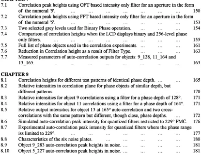
is to perform a multiplication of the input spectrum, F(co), with the Transfer Function

o f the processing system H(co), where H(œ) is the Fourier transform o f h(t).

Fig. 2.1(b).

f(t)

0 h(t)

---m

(b)

Fig. 2.1 The effect of a processing system, h, on a signal,/

(a) in the time domain, (b) in the frequency domain

The output can then be expressed in the time domain if required, by applying the

-1

Inverse Fourier Transform, F .

F'[F(o)]=

jFicoye-^^dco

Equ. 2.3

It is seen that the Fourier transform and inverse Fourier transform are essentially the

same process apart from a change of sign in the exponent. Thus the convolution of

two signals can be performed by taking their Fourier transforms, multiplying, then

(25)

2. 1.3 Th e Cr o s s-Co r r e l a t io n Fu n c t io n

The method o f comparing two signals by Cross-correlation as mentioned above can

be explained in a similar way. The two signals to be correlated replace f(t) and h(t) in

the convolution integral except that one of the signals, h(t) is not reversed before

multiplication and offset, h(t+r).

However, if the signal is complex, then its phase must be reversed, i.e. its complex

conjugate is used in the integral, thus:

f { t ) o h ( t ) = ] f ( T ) . h \ t + r).dT Equ. 2.4

where, h* indicates the complex conjugate of h.

This is called the cross-correlation function, (CCF).

The CCF can therefore be performed on a pair o f functions by reversing one function

on its independent variable and conjugating it before convolving with the other

function. The relation between the two processes can be written as:

f ( t ) o h{t) = [ / ( O 0 }i ( - 0 1 Equ. 2.5

2 2 OPTICAL DIFFRACTION - THE MEANS TO OPTICAL CORRELATION

2.2.1 Ba c k g r o u n d

Over the centuries following the discovery of the wave nature of light, work by

Huygens, Fresnel, Kirchhoff, Rayleigh and Sommerfield eventually led to

mathematical formulations providing effective means to model and predict the

interference effects resulting from diffraction by small apertures. The resulting

interference patterns evolve with distance from the aperture. The application o f scalar

diffraction theories led to the Rayleigh-Sommerfield diffraction formula, equation

Equ. 2.6 which describes the optical amplitude field at any point, Po, after a plane

(26)

(/(PJ= J-rf(/(PjîM M eosZ(n,r„,).<.^

Equ. 2.6

where, U(Po) is the amplitude field at observation point Po,

U(Pi) is the amplitude field at points on the aperture plane,

roi is the distance from Po to a point on the aperture,

Z(n,roi) is the angle between the normal to the aperture and

the vector ro],

À is the wavelength of the light,

k is the wave vector: ilnIX).

This expression is difficult to calculate for practical applications. Fortunately

simplifications can be made if the aperture to observation point distance, | roil, is

large enough. Two zones are identified in which the simplified expressions apply:

a) The Fresnel zone, extends fi"om a distance;

(referred to as the Near Field), to infinity.

b) The Fraunhofer zone, extends from a distance;

(the Far Field), to infinity.

Refer to Fig. 2.2 for co-ordinate notation.

2 . 2 .2 The Fr e s n e la p p r o x im a t io n s

The approximations required to enable the Fresnel diffraction formula to be developed

rely on the introduction of a co-ordinate system in the aperture and observation planes

Fig. 2.2. Points on the observation plane are described by x and}/ co-ordinates while

points in the aperture plane are described by ^ and t] co-ordinates coincident with the

Xand y co-ordinates respectively, apart from a displacement along the z axis, normal

(27)

Direction o f propagation

Diffracting Observation

aperture plane

Fig. 2.2 Co-ordinate system used for the Fresnel approximation

The use of this co-ordinate system allows expression of the cosine term in Equ. 2.6 in

terms of z and roi to provide an alternative version of the Rayleigh-Sommerfield

expression, Equ. 2.7. roi is also eliminated by approximation using the binomial

expansion.

Equ. 2.7

The integral is also extended over infinity rather than just the aperture area as the

aperture's boundaries are implied within its description term U{^,rj). The resulting

Fresnel diffraction expression can be stated in a number of forms, the most familiar

being equations Equ. 2.8 (convolution form) and Equ. 2.9 (Fourier transform form).

For an explanation of how the approximations are applied refer to Appendix A.

Equ. 2.8

U { x . y ) = — e^‘ jX.Z

I , Equ. 2.9

\.e " .d ^ .d r j

2.2.3 Th e FRAUNHOFER A P P R O X IM A T IO N S

When the condition for Fraunhofer diffraction is met the quadratic term in the curly

(28)

can be neglected. The remaining expression is the 2-dimensional Fourier transform of

the aperture function, U{^,rj).

In other words the far field diffraction pattern is the spatial frequency spectrum of the

aperture where the spatial frequencies are:

_ 2 L _ _ Equ. 2.11

A.z ' ' ’ A . z " "

Hence, in the exponential of the Fourier integral:

'Itz

- j — ( x^ + yT]) = - j 2 7 T { s J + Sy7l) = - j { k j + kyîf)

Ignoring the factors outside the integral, the spectrum is:

A detailed examination of the development of these diffraction theories can be found

in reference Goo(bk)96.

It is of course impossible to observe a diffraction pattern at an infinite distance from

the diffracting aperture so a converging lens is placed one focal length from the

diffracting object. When illuminated by monochromatic plane waves the object will

have its image formed at infinity while the Fraunhofer diffraction pattern will appear

one focal length beyond the lens.

2 . 2 . 4 Sp a t ia lfil t er in g

Since the FT represents the spectrum of the spatial frequencies present in an object it

is easy to remove selected spatial frequencies by positioning stops in the Fourier plane

and allowing the remaining components to propagate through the system to form an

image in the usual way.

The 2-dimensional arrangement of stops (whether binary or continuously valued) is

called the Filter. The light field immediately after the Fourier plane is the product of

(29)

transform and the light incident on it is the Fourier transform o f an object placed

before the lens, then the multiplied result may be inverse transformed using a second

lens back into the spatial domain. The light field in the back plane of the second lens,

is then a convolution of the input object and the impulse response represented by the

filter. Fig. 2.3. This is the basis o f the '4f correlator', so-called after the four focal

lengths required for the two successive optical Fourier transforms.

CL .V ■

-c

o

I * 1u %

i

/ /

A

V

/

Fig. 2.3 Schematic diagram of a 4-f Spatial Filter

An extensive theoretical review of this and similar optical configurations for potential

use in signal processing was conducted in the 1950s and 60s by Cutrona et al [C ut60].

However, practical implementation o f the ideas was hindered by the technology

available at the time. Before the advent of the Laser, the coherence lengths of light

sources were relatively short. A coherence length sufficient for interference between

rays traversing the longest and shortest path lengths within the correlator is necessary

for an effective output signal.

2.3 EARLY OPTICAL CORRELATOR DESIGNS

2.3.1 Va n d e r Lu g t Co r r e l a t o r

The first practical implementation o f the 4-f correlator was published by Vander Lugt

[Van64]. The author shows how a complex valued spatial filter can be recorded and

implemented in a 4-f configuration. Established filter design criteria used for

electronic signal processing to detect a known signal in noise states that the greatest

signal to noise ratio at the filter output is achieved by using a 'Matched Filter'. The

(30)

K x , y ) = f \ - x , - y ) _{Equ. 2.14}

Even when the aforementioned optical obstacles were overcome, producing a filter

comprising a complex Fourier transform to match an arbitrary input was not straight

forward. It was not until Vander Lugt suggested a holographic method for recording

a complex filter optically that the '4f correlator' was successfully applied to the

correlation of arbitrary images not described by well defined mathematical functions,

[Van64].

Vander Lugt recorded his complex filter by interfering a tilted plane reference beam

with the optical Fourier transform of the required impulse response by inserting an

impulse response mask (i.e. a representation o f the object to be detected) and Fourier

transform lens into one arm of a Mach-Zehnder interferometer. Fig. 2.4.

Beam splitter

Mirror

Coherent plane wave illumination

Beam splitter

Mirror

Impulse response Recording plane

mask; h(xi,yO applied here

R(x2,y2)+H(x2,y2) y2

Fig. 2.4 Method for recording a Vander Lugt complex filter

The interference pattern is recorded as an intensity function on photographic film.

The intensity exposing any point on the film is dependant on the amplitude and phase

(31)

component to the intensity at the film which, as will be seen is used as a 'carrier

frequency' upon which the diffraction information is held. Goodman, in reference

Goo(bk)96, section 8.4, gives a full explanation. The following is a brief summary of

Vander Lugt’s paper.

The object and reference beams lie in the (y2,z) plane and so that the reference beam's

amplitude at the recording plane, is ro.exp(-j27rocy2), where a=(smQ)/l i.e. its

phase varies with y j according to the tilt of the beam, 9. The reference beam

amplitude and the Transfer function amplitude, {\IXf)H, are vectorially added at that

plane to give an intensity falling on the photographic emulsion, of:

r

+ ^^H .Q xp {j2 n ccy^)

+ -^ H * Q x p (-j2 7 r a y ^ )

where, ro is the reference beam amplitude,

/ i s the focal length of the Fourier transform lens.

The photograph is developed so that its amplitude transmission is proportional to the

intensity which exposed the emulsion, i.e. it's amplitude transmission becomes

proportional to Equ. 2.15, and can be rewritten as:

= + - j ^ A \ x ^ , y ^ ) Equ. 2.16

2 r

+ — ^(x2,y2).cos[2;T(^2 +^^(^2.^2)]

where, A and y/ are the magnitude and phase parts of H,

i.e. H {x„ y;) = A{x„y,)Q xp[j\i/{x^,y,)]

Phase object pattern recognition by optical correlation using a liquid crystal display for spatial phase modulation