Non Linear Submarine Modelling and Motion Control with Model in Loop

Non Linear Submarine Modelling and Motion

Control with Model in Loop

Ashitha1, Ravi Kumar S. T 2, Dr. K Rajesh Shetty 3

M.Tech Student, Dept. of Electronics and Communication, NMAM Institute of Technology, Nitte, Karkala, Karnataka,

India1

Manager, CS/ D&E-NS1, Bharat Electronics Limited, Bangalore, Karnataka, India2

Professor and HOD, Dept. of Electronics and Communication, NMAM Institute of Technology, Nitte, Karkala,

Karnataka, India3

ABSTRACT: This project considers Mathematical Modelling and Control system design of an unmanned underwater vehicle (UUV). It describes the assembly of 6 Degree Of Freedom (DOF) using 6 set of equation of motion and developing a non-linear model for simulation. A nonlinear model of UUV is attained by means of kinematics and dynamics equations which are linear about an execution point to get a straightaway parallel plane model. Control System design involves designing the feed-forward and feedback control laws. The controller help to stipulate to the desired depth and continue at the same depth thereafter. Environmental disturbances are also considered and modelled accordingly.

KEYWORDS: UUV, DOF, Modelling, Control.

I. RELATED WORK

The year 1578 is dated for theoretical design of the submarine in history. The first self propelled torpedo was designed in the year 1868. The main use was found in the off shore gas and oil mining function which was gradually approved by the army and navy for the defence purpose and also for the commercial purpose for the rigorous operation UUV were used. AUV were used by scientist in the study of ocean and ocean floors with the help of thermistor, multi beam echo sounder etc.,. The rapid development in underwater sensors, battery and other supporting technologies, the development of AUV has gained acceleration in recent decades

II. INTRODUCTION

UUV's are Independent Vehicles (Un-tethered) which are battery powered and lies between Remotely Operated Vehicle's (ROV's) (Tethered) and Torpedo. The location and alignment of the UUV are determined in 3 Dimension space and time using 6 DOF. Also, control forces are realized and analysed using 6 DOF equations of motion of a submerged vehicle. The chief forces that act on the vehicle are collective to build the hydro dynamic performance of the body. These key forces are Inertial, Gravitational, Hydro static, Hydrodynamic [2].

III. OBJECTIVE OF THE PROJECT

 To design, develop and test the underwater vehicle with the mathematical model.

 Design the control system for the above mentioned model to maintain the depth of the UUV at the desired

height and maintain it throughout the assigned work is done.

 Designing the model to work even when there is environmental disturbances.

IV. MODELLING

The motion of the UUV is limited to the underwater so we consider the nonlinear equation of motion by the Naval Post Graduation School for AUV II which specifies the 6 DOF. These equation mainly constitute of the hydrodynamic co-efficient, Gravity, Mass together represented as the equation which helps the UUV to progress about in 6 direction. The direction primarily are surge, sway, heave, roll, pitch, yaw. Former 3 represent the linear motion and the latter 3

represent the rotational motion about the linear axis represented as [u, v, w, φ, θ, ψ] respectively. Modelling can also be

derived into two category namely, Kinematics and the Dynamics, where Kinematics deals with the geometrical aspect of the motion where as the dynamics deals with the study of force which results in the motion [5]. The representation of the notation of the UUV is shown in the Table 1.

Table 1: Notation term used while modelling UUV [3]

DOF 1 2 3 4 5 6

Movement Motion

control

in x-axis

(surge)

Motion control

in y-axis

(sway)

Motion control

in z-axis

(heave)

Rotation about x-axis (roll)

Rotation about y-axis (pitch)

Rotation about z-axis (yaw)

Linear and

angular velocity

u v w p q r

Position x y z φ θ ψ

i. Development of the UUV equation of motion

Modelling is performed for different purposes, i.e., sensor model, designing the controller etc. Therefore mathematical modelling of UUV highly relays on fluid's characteristic through which it is moving, vehicle's geometry, feature. To be aware of equation we must understand reference frame.

ii. Reference frame

Body fixed frames: The co-ordinates are suitably fixed to vehicle. The origin is frequently selected to be at major plane

of symmetry of the body [4].

X-axis: directed to right of the vehicle. Y-axis: directed to the front of the vehicle. Z-axis: Orthogonal to X and Y axis.

Local frame: The co-ordinate frame taking fixed star into consideration. The origin is centre of mass of the earth. This

is also called as ENU frame.

Z or U: directed to upwards along ellipse.

X or E : directed to horizontal axis or East direction. Y or N: It is horizontal plane pointing to the North.

To deal with the modelling of the equation of motion we have to deal with converting the ENU frame to the body frame.

ENU to Body transformation

The navigation parameter from the vehicle is obtained by the Inertial Measurement Unit (IMU) and gyroscope these helps to find the position and the orientation of the vehicle practically. But theoretically the 6 DOF of the vehicle helps to find the acceleration with respect to body centred plane, for the help of computation it is converted to the earth centred frame [6]. The equation (1) shows the relation between the ENU frame and the conversion of it to other.

( , , ) = , , , (1)

Exploitation of Euler Angles allows the change from the existing coordinate frame to other in the Cartesian coordinate

changed in relation to the z-axis, then altered about the y-axis, and in the end about the x-axis. Individual matrices are shown in equation (2), (3) and (4).

, =

cos( ) sin( ) 0

−sin( ) cos( ) 0

0 0 1

(2)

, =

cos

( )

( )

0 1 0

sin

( )

( )

(3)

, =

1 0 0

0 cos

( )

( )

0 sin

( )

( )

(4)

Combining of equation (2), (3) and (4) gives equation (5).

( , , ) =

( )cos( ) −sin( ) cos( ) + ( )sin( )sin( ) sin( ) cos( ) + ( )cos( )sin( )

( )cos( ) cos( ) cos( ) + ( )sin( )sin( ) −cos( ) sin( ) + ( )cos( )sin( )

−sin( ) cos( ) sin( ) cos( ) cos( )

The conversion format is given in equation (6) using equation (5).

=R ( , , )

̇

̇

̇

(6)

Similarly for the rotational term conversion is given by as shown in equation (7) in detail.

=

1 0 −sin( )

0 cos( ) sin

( )

0 −sin( ) cos

( )

̇

̇

̇

(7)

The conversion matrices are known as Directional Cosine Matrix (DCM).

iii. Equation of motion

The equations of motion is primarily derived from the Newton's 2nd Law related to acceleration. i.e.,

= (8)

where, is the force, is the mass, is the acceleration.

For 6 degrees of freedom of the vehicle, the geological position, , and and Euler angles , and can be

represented in vector form as in equation (10)

= [ ] (9)

the linear and angular velocity of the body fixed frame are represented as in equation (11)

= [ ] (10)

The final 6 DOF is given by using the equation shown equation (12)

where, is the mass matrix here is divided into and i.e., added mass and rigid body mass respectively.

= + (12)

Rigid body mass is due to the static vehicular body mass and added mass is the extra mass added to the vehicle when it is submerged in the sea.

In equation (11), stands for the Coriolis and the Centripetal forces. These are basically a apparent forces but affect

the motion dynamics of the equation so it is considered for the computing. as with the mass matrix consists of two

matrices, and , summed together,

= + (13)

is the rigid body Coriolis and centripetal matrix is tempted by , while is a Coriolis-like matrix made by .

In equation (11), refers the hydrodynamic damping matrix. The damping matrix consists of the drag and lift of the vehicle due to hydrodynamic co-efficient, which is shown in equation (14).

( ) = ⎣ ⎢ ⎢ ⎢ ⎢ ⎡ + | || | 0 0 0 + | || | 0 0 0 + | || | 0 0 0 0 0 0 0 0 0 0 0 0 0 0 0 0 0 0 + | || | 0 0 0 + | || | 0 0 0 + | || |⎦ ⎥ ⎥ ⎥ ⎥ ⎤ (14)

In equation (11), represent the restoring forces and the moments. The restoring force and moment constitute of the gravitational force and the buoyancy of the vehicle which is the function of the vehicles mass.

= +

x + x (15)

While is the centre of buoyancy and is the centre of gravity or mass in frame.

=

(

)

0 0 −

, where = ∇ (16)

Here is the buoyant force vector caused by buoyancy, is gravity constant 9.81m/s2 , is fluid density, is the

fluid displaced by the AUV [m3]

=

(

)

0

, where = (17)

is the gravitational force vector caused by the AUV. Combining equation (16) and (17) substituting in (15) we get

equation (18). = ⎣ ⎢ ⎢ ⎢ ⎢ ⎡ ( − ) −( − ) −( − ) ( − ) ( + ) − ( + )⎦ ⎥ ⎥ ⎥ ⎥ ⎤ (18)

V. CONTROL PROBLEM

The advancement in UUV increases these vehicle popularity worldwide. There was a great demand for the design of the controller. The uncomplicated form of algorithm in PID controller is P controller. P controller's major practice is to reduce the steady state error. To even out the uneven course P controller is chiefly used in course of first order with

single energy storage. As the gain factor K raises, the steady state inaccuracy of the diminishes in the scheme. Though,

in spite of the decrease, P control can certainly not handle to remove the steady state error of the system. This controller can be employed only when our structure is tolerable to a invariable steady state error. Also, without difficulty it is justified that affect after a certain value of diminution on the steady state error and P controller reduces the increase time, system response overshoots by growing of . P controller is evaluated as in (19).

( ) = + ( ) (19)

where, 0 is the initial value, is the proportionality constant, ( ) error which is the function of the desired value and

the obtained output.

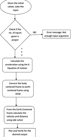
Figure 1: Flowchart to find the distance travelled by UUV using equation of motion.

VI. RESULTS

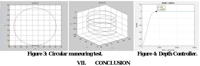
To validate the 6 DOF equations of motion pertaining to the modelling of AUV, inputs are given with respect to Surge velocity and rudder angle which results in circular Manoeuvring as shown in Figure 3. The Depth controller of the UUV is as shown in Figure 4, where the depth is controlled to desired height and there after maintaining the same depth.

Figure 3: Circular maneuring test. Figure 4: Depth Controller.

VII. CONCLUSION

Modelling of AUV using six DOF gives us the control over six dimensions of vehicle motion. This increases the stability of vehicle over natural disturbances during the motion of vehicle and thus reflecting the real behaviour of the vehicle which acts under water. The P controller is verified for various proportionality constants and for various depths, the raise and dawn motion of the UUV can be observed in the results.

REFERENCES

[1] Brooks Louis-Kiguchi Reed, “Controller Design for Underwater Vehicle Systems with Communication Constraints", Submitted to the Joint Program in Applied Ocean Science and Engineering, 2014.

[2] Miroslaw Tomera, “Nonlinear controller design of a ship autopilot”, International Journal of Applied Mathematics Computer Science, Vol. 20 No. 2, 271-280 pp. , 2010.

[3] Thor I. Fossen, “Guidance and Control of Ocean Vehicles", University of Trondheim Norway, 1994.

[4] Xiao Liang, Yongjie Pang, Lei Wan and Bo Wang, “Dynamic Modelling and Motion Control for Underwater Vehicles with Fins", International Technology of Vienna,Vol.28, 539-556 pp. , 2008.

[5] Xiao Liang, Jundong Zhang, Yu Qin and Hongrui Yang, “Dynamic Modeling and Computer Simulation for Autonomous Underwater Vehicles with Fins", Journals of Computer, Vol. 8, No. 4, 1058-1064pp. , 2013.

[6] J. H. A. M Vervoort, “Modelling and Control of Unmanned Underwater vehicle JHAM Vervoort” , 2008.