Quantile-Based Permutation Thresholds for Quantitative Trait Loci Hotspots

(1)

INVESTIGATION

Quantile-Based Permutation Thresholds

for Quantitative Trait Loci Hotspots

Elias Chaibub Neto,* Mark P. Keller,†_{Andrew F. Broman,}†_{Alan D. Attie,}†_{Ritsert C. Jansen,}‡

Karl W. Broman,§_{and Brian S. Yandell**},††,1 *Department of Computational Biology, Sage Bionetworks, Seattle, Washington 98109,†Department of Biochemistry, §_{Department of Biostatistics and Medical Informatics, **Department of Statistics, and}††_{Department of Horticulture, University of} Wisconsin, Madison, Wisconsin 53706, and‡Groningen Bioinformatics Centre, Groningen Biomolecular Sciences and Biotechnology Institute, University of Groningen, Nijenborgh 7, Groningen, The Netherlands

ABSTRACTQuantitative trait loci (QTL) hotspots (genomic locations affecting many traits) are a common feature in genetical genomics studies and are biologically interesting since they may harbor critical regulators. Therefore, statistical procedures to assess the significance of hotspots are of key importance. One approach, randomly allocating observed QTL across the genomic locations separately by trait, implicitly assumes all traits are uncorrelated. Recently, an empirical test for QTL hotspots was proposed on the basis of the number of traits that exceed a predetermined LOD value, such as the standard permutation LOD threshold. The permutation null distribution of the maximum number of traits across all genomic locations preserves the correlation structure among the phenotypes, avoiding the detection of spurious hotspots due to nongenetic correlation induced by uncontrolled environmental factors and unmeasured variables. However, by considering only the number of traits above a threshold, without accounting for the magnitude of the LOD scores, relevant information is lost. In particular, biologically interesting hotspots composed of a moderate to small number of traits with strong LOD scores may be neglected as nonsignificant. In this article we propose a quantile-based permutation approach that simultaneously accounts for the number and the LOD scores of traits within the hotspots. By considering a sliding scale of mapping thresholds, our method can assess the statistical significance of both small and large hotspots. Although the proposed approach can be applied to any type of heritable high-volume“omic”data set, we restrict our attention to expression (e)QTL analysis. We assess and compare the performances of these three methods in simulations and we illustrate how our approach can effectively assess the significance of moderate and small hotspots with strong LOD scores in a yeast expression data set.

Q

UANTITATIVE trait loci (QTL) hotspots, groups of traits comapping to the same genomic location, are a common feature of genetical genomics studies. Genomic locations associated with many traits are biologically interesting since they may harbor inﬂuential regulators. Therefore, statistical procedures aiming to assess the signiﬁcance of such hotspots are of key importance.

Brem et al. (2002) and Schadt et al. (2003) detected

hotspots by dividing the genome of an organism into equally spaced bins, counting the number of expression traits with

a QTL in each bin. A hotspot was considered signiﬁcant if it had more traits with QTL than expected if the expression QTL were randomly distributed across the genome. Darvasi (2003) and Perez-Enciso (2004) pointed out that these hot-spots may arise as an artifact of high correlation among expression traits, rather than by the action of a common master regulator. Nongenetic mechanisms, uncontrolled en-vironmental factors, and unmeasured variables are capable of inducing strong correlations among clusters of traits. Hence, whenever a trait shows a spurious linkage, many correlated traits will likely map to the same locus, creating a spurious expression (e)QTL hotspot. Furthermore, multi-ple-testing and relaxed-mapping thresholds may inﬂate the hotspots (Darvasi 2003).

Westet al.(2007) and Wuet al.(2008) proposed a

doi: 10.1534/genetics.112.139451

Manuscript received February 8, 2012; accepted for publication May 18, 2012 Available freely online through the author-supported open access option. Supporting information is available online at http://www.genetics.org/content/ suppl/2012/06/01/genetics.112.139451.DC1.

(2)

by trait, using the distribution of the maximal number of expression traits across the genome to assess hotspot signif-icance. ThisQ-method permutes QTL positions, not pheno-type or genopheno-type data, and improves upon the permutation approaches of Brem et al.(2002) and Schadt et al.(2003) since it accounts for multiple testing across the genome. However, theQ-method implicitly assumes traits are uncor-related and hence underestimates the clustered pattern of spurious eQTL for correlated traits.

Breitling et al.(2008) proposed a permutation test that randomized rows in the marker data relative to rows in the trait data, preserving the correlation structure among phe-notypes. The null distribution for thisN-method of hotspot sizes depends on the number N of traits with LOD score exceeding a predetermined LOD threshold at each locus. The choice of LOD threshold is important: higher LOD thresholds yield smaller-sized spurious hotspots by chance under the null hypothesis of no hotspots. Two natural LOD threshold choices are the Churchill–Doerge (Churchill and Doerge 1994) single-trait LOD threshold, controlling genome-wide error rate (GWER) for one trait, and a conservative permutation threshold for the maximum LOD score across all traits and all genomic locations. The former allows large hotspots by chance under the null distribution (Breitling

et al. 2008). The latter favors small hotspots composed of

traits with high LOD scores under the null. Which threshold is more appropriate?

We propose a quantile-based permutation approach, the

NL-method, with a sliding scale of thresholds ranging from the conservative to the single-trait threshold, jointly consider-ing hotspot size and the distribution of LOD scores among correlated traits. Hence, even a small hotspot, with a modest number of correlated traits all having high LOD scores at a location, can be signiﬁcant. The NL-method controls the genome-wide error rate across a range of possible hotspot sizes. Explicitly, we examine spurious hotspot sizen, ranging from 1 toN, withNthe hotspot size threshold delivered by theN-method using the single-trait LOD threshold. While the

N-method yields the minimum signiﬁcant hotspot size for aﬁxed LOD threshold, we turn the problem around and deter-mine an empirical LOD threshold given a spurious hotspot size. We assessed and compared the performances of theNL-,

N-, andQ-methods using (i) simulated examples, where we generated hotspots with varying LOD-score distributions for data sets with correlated and uncorrelated traits, and (ii) simulation studies, where we generated null data sets, i.e., data sets where none of the phenotypes had any QTL, and assessed the error rates of the three procedures under dif-ferent levels of correlation among the traits. Application of theNL-method to a yeast data set detected additional mod-erate and small hotspots considered nonsigniﬁcant by the

N-method and avoided spurious hotspots detected by the

Q-method. This ability to assess the statistical signiﬁcance of hotspots with varying sizes and LOD-score distributions has the potential to yield important additional biological discoveries.

Methods

The Q- and N-methods

The now standard permutation threshold method for QTL mapping (Churchill and Doerge 1994) estimates the null distribution of the genome-wide maximum LOD score by shufﬂing the phenotypes relative to the genotype data, breaking the association between the phenotype and the genotypes. Our interest, though, is to assess the signiﬁcance of QTL hotspots. This section presents two different permu-tation schemes that have been used in hotspot analysis.

Supporting Information, Figure S1 shows a schematic of

the genotype data, the phenotype data, and the output of hotspot analysis in genetical genomics experiments.

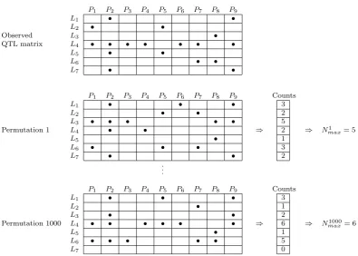
Theﬁrst permutation scheme for theQ-method (Figure S2) derives the null distribution of hotspot sizes by permuting the cells of the observed QTL matrix along its rows, independently for each column; that is, the QTL are permuted across geno-mic locations separately by trait. TheQ-method does not ac-count for the correlation structure among the phenotypes and, contrary to the Churchill–Doerge and Breitling’s permutation tests, does not break the connection between phenotypes and genotypes. The Q-method permutation null distribution is generated under the assumption that phenotypes are uncor-related. Violation of this assumption leads to a severe under-estimation of the null distribution of hotspot sizes and to detection of many spurious hotspots, as shown by Breitling

et al. (2008) in the reanalysis of the Wu et al. (2008) data

and illustrated in the simulation study and examples below. The second permutation scheme (Breitling et al. 2008) (Figure S3) used for theN- andNL-methods breaks the con-nection between genotypes and phenotypes while preserving the correlation structure separately within each of the types of data by permuting the rows of the phenotype data matrix relative to the rows of the genotype data. Mapping analysis is redone for all traits with the permuted data. This scheme, a direct extension of Churchill and Doerge (1994), preserves the correlation structure among the phenotypes, accounting for spurious hotspots due to nongenetic correlation.

The NL-method

In linkage analysis of a single phenotype we are usually interested in controlling the GWER of falsely detecting a QTL. For a given error ratea, we determine a single-trait mapping LOD thresholdlsuch that

Pr max

k fLODkg$ljthere is no QTL anywhere in the genome

¼a;

(1)

(3)

Prðmax

t;k

LODt;k

$lcjnone of the traits have a QTL anywhere in the genomeÞ ¼a;

(2)

wheret= 1,. . .,T,k= 1,. . .,K, andlcrepresents a more

conservative LOD threshold that controls the probability that any of the traits have one or more false linkages any-where in the genome.

Which threshold is more adequate depends on the underlying situation. We discard small hotspots with strong LOD scores when we adopt l, but we miss hotspots com-posed of many traits with linkages barely reaching the sin-gle-trait mapping threshold usinglc. Therefore, we propose

a sliding scale of thresholdsln,afornvarying from 1 toN, where N represents the hotspot size (i.e., the number of traits with signiﬁcant LOD at a given genomic location) expected by chance under the N-method’s permutation scheme, computed using the LOD-score thresholdl.

Given a ﬁxed mapping threshold, the N-method deter-mines the hotspot size expected by chance. We turn the problem around: given aﬁxed spurious hotspot sizen, the

NL-method determines the associated mapping threshold ln,a. We adopt maxk{qLODk(n)} as a test statistic where qLODk(n) corresponds to thenth LOD value of an ordered sample of T LOD scores, ordered from highest to lowest. Note that by taking the maximum of qLODk(n) across the genome we are able to control the genome-wide error rate associated with the qLODk(n) statistic. Explicitly, we control

Prðmax

k fqLODkðnÞg

$ln_;ajnone of the traits have a QTL anywhere in the genomeÞ

¼a:

(3)

In other words, by adopting a QTL mapping thresholdln,awe control GWER at level a of detecting at least one spurious hotspot of sizenor higher somewhere in the genome, given that none of the traits have a QTL anywhere in the genome. Observe that when n = N, the LOD threshold l (that controls the detection of a false QTL at a GWERa) matches lN,a(that controls the detection of a false hotspot of sizeN or higher), and qLODk(N) corresponds to LODk. Therefore, when n=N, the quantity in (3) reduces to (1). Similarly, when n = 1, we have that lc = l1,a and qLODk(1) = maxt{LODt,k}, so that maxk{qLODk(1)} = maxt,k{LODt,k} and (3) reduces to (2).

Finally, the quantity in (3) is the probability of detecting at least one spurious hotspot ofsize exactly nsomewhere in the genome given that none of the traits have a QTL anywhere in the genome. However, under the null hypothesis of no QTL, detecting a hotspot of sizen*.nis less likely than detecting a hotspot of sizen; therefore, if a thresholdln,acontrols the full-null GWER for a hotspot of sizen, it will also control the full-null GWER for a hotspot of size larger thann. Below, we detail the permutation algorithm for LOD quantiles.

NL-method algorithm:For aﬁxed hotspot size,n= 1,. . .,

N, we obtain the permutation LOD threshold that controls the genome-wide error rate of detecting at least one hotspot of sizenor higher, at aﬁxedalevel as follows:

1. Permute the data according to theN-method to break the associations among genotypes and phenotypes, while keeping the correlation structure among phenotypes in-tact. Compute the LOD scores for all phenotypes across all genomic locations.

2. Process the LOD proﬁle of each trait as follows: (i) de-termine the LOD peak for each chromosome, (ii) compute the LOD support interval around the peak (Lander and Botstein 1989; Dupuis and Siegmund 1999; Manichaikul

et al.2006), and (iii) set to zero the LOD scores outside

the LOD support interval (and below the single-trait map-ping threshold).

3. For aﬁxed hotspot sizen, compute qLODk(n) for genomic positionsk= 1,. . .,Kand store its maximum.

4. Repeat steps 1–3,B times. The histogram of the B -per-mutation samples of maxk{qLODk(n)} is an estimate of the null distribution of the test statistic for at least one spurious hotspot of size n or higher anywhere in the genome, given that none of the traits have a QTL any-where in the genome.

5. The upper (1 2a)-quantile of the permutation sample generated in step 4 is our threshold (denoted byln,a).

This algorithm is analogous to the traditional permuta-tion test, replacing LOD scores by LOD quantiles. Chen and Storey (2006) perform permutation tests for distinct quantile-based statistics, in a different context, where they consider a set of relaxed signiﬁcance thresholds to detect multiple QTL for a single trait.

The LOD-score processing step described in step 2 of the

(4)

p. 231). Permutation tests remain valid for a multivariate re-sponse that can be reduced to a single-valued test statistic (Good 1994, Chap. 5). Exchangeability of subjects under the null distribution follows by the construction of an exper-imental cross. At a ﬁxed genomic location our test statistic corresponds to qLODk(n). Across the whole genome, we adopt maxk{qLODk(n)} as our genome-wide and single-valued test statistic.

Results

Simulated examples

In this section we illustrate the application of theQ-,N-, and

NL-methods to two simulated data sets: one with highly correlated traits and the other with uncorrelated traits. We generated data from backcrosses composed of 112 individ-uals with 16 chromosomes of length 400 cM containing 185 equally spaced markers each, and phenotype data on 6000 traits. The phenotype data were generated according to the models

Yk¼bMþuLþek; if Yk belongs to a hotspot;

Yk¼uLþek; if Yk does not belong to a hotspot; whereLN(0,s2_{) represents a latent variable that affects}

all k = 1,. . ., 6000 traits; u represents the latent variable

effect on the phenotype and works as a tuning parameter to control the strength of the correlation among the traits;M= gQ+eMrepresents a master regulator trait that affects the phenotypes in the hotspot;brepresents the master regulator effect on the phenotype; and Q represents the QTL giving rise to the hotspot. Note that traits composing the hotspot are directly affected by the master regulatorMand map toQ

indirectly,grepresents the QTL effect on the master regula-tor, and ek and eM represent independent and identically distributed error terms following aN(0,s2_{) distribution.}

In both examples we simulated three hotspots: (i) a small hotspot located at 200 cM on chromosome 5 showing high LOD scores (see Figure S5, A and D), (ii) a big hotspot located at 200 cM on chromosome 7 showing LOD scores ranging from small to high (seeFigure S5, B and E), and (iii) a big hotspot located at 200 cM on chromosome 15 showing LOD scores ranging from small to moderate (seeFigure S5, C and F).

In both simulations we sets2_{= 1 and}_g_{= 2. QTL}

anal-ysis was performed using Haley–Knott regression (Haley and Knott 1992) with the R/qtl software (Broman et al.

2003). We adopted Haldane’s map function and genotype error rate of 0.0001. Because we adopted a dense genetic map (our markers are2.16 cM apart), we did not consider putative QTL positions between markers.

In the ﬁrst example, denoted simulated example 1, we adopted a latent effect of 1.5. In the second example, denoted simulated example 2, we adopted a latent effect of 0 and simulated uncorrelated traits. Figure S6, A and B, shows the distribution of all pairwise correlations among

the 6000 traits for both simulated examples. These extreme examples illustrate the effect of phenotype correlation on QTL hotspot sizes. The correlations of the real data are ac-tually intermediate (seeFigure S6C).

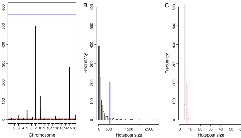
Figure 1 shows the results for theQ- andN-methods for simulated example 1, usinga= 0.05. Figure 1A shows the hotspot architecture computed using a single-trait LOD threshold of 3.65; i.e., at each genomic location the plot shows the number of traits with LOD score.3.65. In addi-tion to the simulated hotspots on chromosomes 5, 7, and 15, Figure 1A shows a few spurious hotspots, including a big hotspot on chromosome 8. The blue and red lines show the

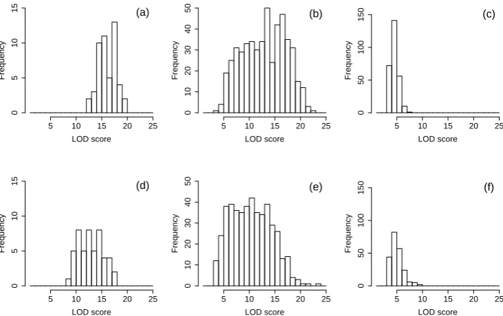
N- and Q-methods’thresholds, 560 and 7, respectively. In this example the N-method was unable to detect any hot-spots, whereas the Q-method detected false hotspots on chromosomes 3, 6, 8, 9, 12, and 16. Figure 1, B and C, shows the hotspot size null distributions and the 5% signif-icance thresholds for theN- andQ-methods, respectively.

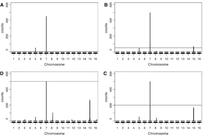
Figures 2 and 3 show theNL-method analysis results for simulated example 1, using a = 0.05. Figure 2, A–D, presents the hotspot architecture inferred using four different quantile-based permutation thresholds. Figure 2A presents the hotspot architecture inferred using a LOD threshold of 7.07. Only the true hotspots (on chromosomes 5, 7, and 15) were signiﬁcant by this conservative threshold. Figure 2B presents the hotspot architecture computed using a LOD threshold of 4.93 that aims to control GWER # 0.05 for spurious hotspots of size 50. The hotspots on chromosomes 5, 7, and 15 were detected by this threshold. Figure 2, C and D, shows the hotspot architectures using LOD thresholds of 4.21 and 3.72, respectively. Only the hotspot on chromosome 7 was detected as signiﬁcant for these thresholds. Note that neither the big spurious hotspot on chromosome 8 nor any of the other spurious hotspots shown in Figure 1A were picked up by the quantile-based thresholds.

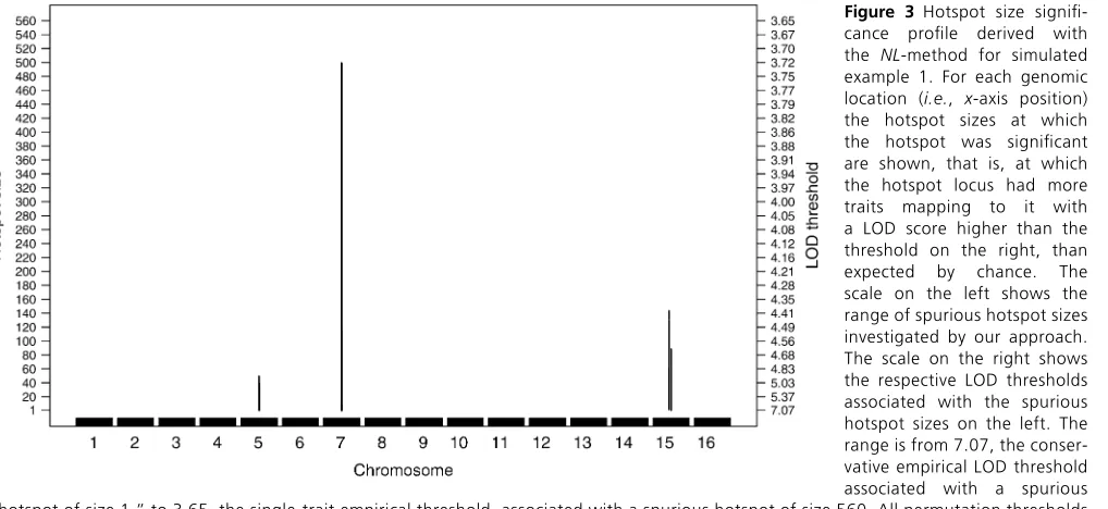
Figure 3 connects hotspot size to quantile-based thresh-old. This hotspot size signiﬁcance proﬁle depicts a sliding window of hotspot size thresholds ranging fromn= 1,. . .,

N, whereN= 560 corresponds to the hotspot size threshold derived from theNmethod. For each genomic location, the hotspot size (left axis) is significant for the LOD threshold (right axis). For example, the chromosome 5 hotspot was significant up to size 49, meaning that.1 trait mapped to the hotspot locus with LOD.7.07,.2 traits mapped to the hotspot locus with LOD.6.46, and so on up to hotspot size 49 where.49 traits mapped to the hotspot locus with LOD .4.93. The hotspot on chromosome 7 was significant up to size 499, and the hotspot on chromosome 15 (higher peak) was significant for hotspot sizes 2–129 and 132–143.

(5)

important, theNL-method dismissed spurious hotspots, such as chromosome 8, composed of numerous traits with LOD scores,5.57.

Figure 4 shows the results for theQ- andN-methods for simulated example 2, usinga= 0.05. Figure 4A shows the hotspot architecture. The blue and red lines show theN- and

Q-method’s thresholds, 19 and 8, respectively. In this exam-ple, both the N- andQ-methods were able to correctly pick up the hotspots on chromosomes 5, 7, and 15.

Comparison of Figures 1A and 4A shows that the spurious hotspots tend to be much smaller when the traits are uncorre-lated (compare chromosome 8 on both plots), leading to much smaller N-method thresholds (compare the blue lines). The

Q-method thresholds, on the other hand, are quite close. This is expected since theQ-method threshold depends on the num-ber of significant QTL (we observed 3162 significant linkages in simulated example 1, against 3586 significant linkages in example 2) and not on the correlation among the traits.

Figure S7displays the hotspot size signiﬁcance proﬁle for

simulated example 2. TheNL-method also detected the hot-spots on chromosomes 5, 7, and 15.

Simulation study

In this simulation study we assess and compare the error rates of theQ-,N-, andNL-methods under three different levels of correlation among the traits. To determine whether the meth-ods are capable of controlling the GWER at the target levels, we conduct separate simulation experiments as follows:

1. We generate a “null genetical genomics data set” from a backcross composed of (i) 6000 traits, none of which is affected by a QTL, but that are nevertheless affected by a common latent variable to generate a correlation structure among the traits, and (ii) genotype data on 2960 equally spaced markers across 16 chromosomes of length 400 cM (185 markers per chromosome). Any detected QTL hotspot is spurious, arising from correlation among the traits. 2. We perform QTL mapping analysis, and 1.5-LOD support

interval processing, of the 6000 traits. For each one of the following single-trait QTL mapping permutation thresh-olds (that control GWER at thea= 0.01, 0.02,. . ., 0.10 levels, respectively), we do the following:

a. We compute the observed QTL matrix and generate theQ-method hotspot size threshold on the basis of 1000 permutations of the observed QTL matrix. We record whether or not we see at least one spurious hotspot of size greater than theQ-method threshold anywhere in the genome.

b. For each genomic location we count the number of traits above the single-trait LOD threshold. We compute the N-method hotspot size threshold on the basis of 1000 permutations of the null data set. We record whether at least one spurious hot-spot of size greater than theN-method threshold is anywhere in the genome.

c. We compute the NL-method LOD thresholds for spurious hotspot size thresholds ranging from 1

(6)

to the N-method threshold. For each NL-method LOD threshold,ln,a, wheren= 1,. . .,N, we count,

at each genomic location, how many traits mapped to that genomic location with a LOD . ln,a and record whether there is at least one spurious hotspot of size greater thannanywhere in the genome.

3. We repeat theﬁrst two steps 1000 times. For each one of the three methods, the proportion of times we recorded spurious hotspots, out of the 1000 simulations, gives us an estimate of the empirical GWER associated with the method.

QTL analysis was performed as described above. Figure 5 shows the simulation results for null data sets gener-ated using latent variable effects of 0.0, 0.25, and 1.0. The Q- and N-methods, with observed GWER (red), and target error rate (black), have two a-levels, a1 for QTL

mapping anda2for the tail area of the hotspot size

permu-tation null distribution. Figure 5 displays the results when a1=a2= 0.01, 0.02,. . ., 0.10. TheNL-method has a single

a-level; the red curves are the observed GWERs for spurious hotspot sizesn= 1,. . .,N, whereNrepresents theNmethod’s permutation threshold.

Figure 5, A–C, shows that for uncorrelated traits theQ- and

N-methods were conservative, below target levels, whereas theNL-method shows error rates about the right target levels

for most hotspot sizes. Figure 5, D and G, shows that error rates for the Q-method are higher than target levels when the traits are correlated and increase with correlation strength among the phenotypes. These results are expected since the Q-method’s thresholds depend on the number of QTL detected in the unpermuted data and tend to increase with the number of phenotypes. Because we generated the same number of phenotypes in the three simulation studies, theQ-method’s thresholds were similar. Therefore, the num-ber and the size of the spurious QTL tend to be proportional to the correlation strength of the phenotypes. The N- and

NL-methods, on the other hand, are designed to cope with the correlation structure among the phenotypes and show error rates close to the target levels as shown in Figure 5, E, F, H, and I.

Yeast data set example

In this section we illustrate and compare the Q-, N-, and

NL-methods using data generated from a cross between two parent strains of yeast: a laboratory strain and a wild isolate from a California vineyard (Brem and Kruglyak 2005). The data consist of expression measurements on 5740 transcripts measured on 112 segregant strains, with dense genotype data on 2956 markers. Processing of the expression measurements of raw data was done as described in Brem and Kruglyak

(7)

(2005), with an additional step of converting the processed measurements to normal quantiles by the transformation

F21_½ð

ri20:5Þ=112, whereFis the standard normal cumu-lative density function, and the ri are the ranks. We per-formed QTL analysis using Haley–Knott regression (Haley and Knott 1992) with the R/qtl software (Broman et al.

2003). We adopted Haldane’s map function, with a geno-type error rate of 0.0001, and set the maximum distance between positions at which genotype probabilities were calculated to 2 cM.

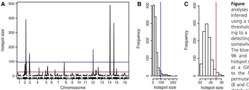
Hotspot analysis of the yeast data, based on theN-method (Figure 6A), detected significant eQTL hotpots on chromo-somes 2 (second peak), 3, 12 (first peak), 14, and 15 (first peak), at a GWER of 5% according to null distribution of hot-spot sizes shown in Figure 6B. The blue line represents theN

method’s significance threshold ofN= 96. The maximum hot-spot size on chromosome 8 was 95 and almost reached signif-icance. Nonetheless, Figure 6A also shows suggestive (although substantially smaller) peaks on chromosomes 1, 4, 5, 7, 9, 12 (second peak), 13, 15 (second peak), and 16 that did not reach significance according to theN-method’s significance threshold. The red line in Figure 6A represents theQ-method’s sig-nificance threshold of 28, derived from the null distribution of hotspot sizes shown in Figure 6C. TheQ-method detected significant hotspots on chromosomes 2 (both peaks), 3, 4, 5 (both peaks), 7, 8, 12 (both peaks), 13, 14, and 15 (both peaks).

Figure 7 shows the hotspot signiﬁcance proﬁle for the

NL-method. The major hotspots on chromosomes 2, 3, 12 (first peak), 14, and 15 (first peak) were significant across all thresholds tested up, and the hotspot on chromosome 8 was significant up to size 93. Furthermore, theNL-method showed that the small hotspots detected by the Q-method on chromosomes 5, 12 (second peak), 13, and 15 (second

peak) might indeed be real. Nonetheless, the small hotspots on chromosomes 4 and 7, detected by the Q-method, are less interesting than the small hotspot on chromosome 1 that was actually missed by theQ-method.

Discussion

A common feature in genetical genomics studies of expres-sion traits is the presence of eQTL hotspots where a single polymorphism leads to widespread downstream changes in the expression of distant genes. These genomic loci associ-ated with many distant genes are biologically interesting since they may harbor important regulators. Statistical procedures aiming to assess the signiﬁcance of such hotspots are of key importance.

Breitlinget al.(2008) were theﬁrst to propose a permu-tation test (theN-method) for eQTL hotspots that accounts for the correlation structure among phenotypes due to the effect of confounders. However, the authors restricted their attention to the single-trait empirical threshold only and may have overlooked interesting hotspots composed of mod-erate to small numbers of traits with strong LOD scores.

In this article, we adopt the Breitlinget al.permutation scheme and propose a method to determine a range of quantile-based permutation thresholds (theNL-method) that allows us to assess the significance of hotspots on the basis of the number and the linkage strength of the traits composing those hotspots. For afixed error ratea, our approach inves-tigates the significance of a hotspot, using a range ofN dis-tinct mapping thresholds, whereNis the smallest hotspot size that is significant by theN-method. For eachn= 1,. . .,Nwe determine the LOD threshold that controls the genome-wide error rate of detecting at least one spurious hotspot of sizen

or higher somewhere in the genome, at an error rate#a.

Figure 3 Hotspot size signiﬁ

-cance proﬁle derived with

the NL-method for simulated

example 1. For each genomic location (i.e., x-axis position) the hotspot sizes at which

the hotspot was signiﬁcant

are shown, that is, at which the hotspot locus had more

traits mapping to it with

a LOD score higher than the threshold on the right, than

expected by chance. The

scale on the left shows the range of spurious hotspot sizes investigated by our approach. The scale on the right shows the respective LOD thresholds associated with the spurious hotspot sizes on the left. The range is from 7.07, the conser-vative empirical LOD threshold

associated with a spurious

(8)

Our simulated examples and simulation studies show that theQ-method performs well when the traits are uncor-related, but detects spurious hotspots at high rates when the traits are correlated. This result is not surprising since the

Q-method implicitly assumes that the traits are uncorrelated.

Molecular traits such as mRNA expression levels, metabolite concentrations, and protein levels are often highly corre-lated and theQ-method is not adequate in these situations. On the other hand, our simulations suggest that the Nand

N- and NL-methods perform adequately for correlated or

Figure 4 N- andQ-method analyses for simulated example 2. (A) Inferred hotspot architecture using a single-trait permutation threshold of 3.65 corresponding to a GWER of 5% of falsely detecting at least one QTL somewhere in the genome. The blue line at count 19 corresponds to the hotspot size expected by chance at a GWER of 5% according to theN-method permutation test. The red line at count 8 corresponds to theQ-method’s 5% signiﬁcance threshold. The hotspots on chromosomes 5, 7, and 15 have sizes 50, 464, and 220, respectively. (B) TheN-method’s permutation null distribution of the maximum genome-wide hotspot size. The blue line at 19 corresponds to the hotspot size expected by chance at a GWER of 5%. (C) TheQ-method’s permutation null distribution of the maximum genome-wide hotspot size. The red line at 8 shows the 5% threshold. Results are based on 1000 permutations.

Figure 5 Observed GWER for theQ-,N-, andNL-methods under varying strengths of phenotype correlation. Black lines show the targeted error rates. Red curves show the observed GWER. (A–C) Results for uncorre-lated phenotypes. (D–F) Results for weakly correlated phenotypes generated using a latent variable effect of 0.25. (G–I) Simulation results for highly correlated phenotypes generated using latent effect set to 1. The left, middle, and right columns show the results for the Q-, N-, and NL-methods, respectively. Note the different y-axis scales for theQ-method panels.

The red curves on the NL-method panels show

(9)

uncorrelated traits, showing genome-wide error rates close the target levels.

The advantage of the NL-method over the N-method is that it can assess the significance of hotspots with any type of LOD-score distribution. For instance, (i) a hotspot com-posed of many traits with moderate LOD scores will be found with thresholds close to the single-trait threshold, (ii) a hot-spot consisting of a few traits with strong LOD scores will be detected with thresholds close to the conservative threshold, and (iii) a large hotspot with a range of moderate to large LOD scores will be significant at all thresholds in our sliding scale. The ability to assess the significance of these different types of hotspots can lead to important additional biological

findings that might be overlooked by previous approaches, while still avoiding the detection of spurious hotspots. In the analysis of the yeast data, the hotspots on chromosomes 5, 8, 12 (second peak), 13, and 15 (second peak) have a LOD distribution of type ii. The hotspots on chromosomes 2, 3, 12 (first peak), 14, and 15 (first peak) have LOD distributions of

type iii. No hotspot with LOD distribution of type i is present in the yeast data set. Note that hotspots composed of moder-ate to small numbers of traits with modermoder-ate LOD scores will be missed by all thresholds in our sliding scale and will be discarded as nonsigniﬁcant by our analysis. Application of the

N-method detected only the ﬁve big hotspots on chromo-somes 2, 3, 12, 14, and 15. Additionally, the simulated exam-ple 1 shows an examexam-ple were theNL-method was able to pick up the three simulated hotspots missed by theN-method.

The NL-method is in a certain sense analogous to the approach proposed by Chen and Storey (2006). In the same way that Chen and Storey relax the single-trait mapping threshold by controlling the probability that a trait falsely maps to kor more genomic locations, we relax the conser-vative threshold by controlling the probability that$ntraits falsely map to a common genomic location.

Even though the sliding window of thresholds delivered by the NL-method method is more informative than the single-hotspot size threshold of the N method, these

Figure 6 N- and Q-method analyses for the yeast data. (A)

Inferred hotspot architecture

using a single-trait permutation threshold of 3.44 correspond-ing to a GWER of 5% of falsely detecting at least one QTL somewhere in the genome. The blue and red lines at counts 96 and 28 correspond to the hotspot size expected by chance at a GWER of 5% according

to the N- and the Q-method

permutation tests, respectively. (B and C) The permutation null distributions of the maximum genome-wide hotspot size based on 1000 permutations. The blue and red lines at 96 and 28 correspond, respectively, to the hotspot size expected by chance at a GWER of 5% for theN- andQ-methods.

Figure 7 Hotspot size signiﬁ -cance proﬁle derived with the

NL-method. The range is from

7.40, the conservative empirical LOD threshold associated with a spurious “hotspot of size 1,”

to 3.45, the single-trait empirical threshold, associated with a spurious hotspot of size 96. All permutation thresholds were

computed targeting GWER #

(10)

approaches have the same computational complexity. They use exactly the same permutations but summarize the results differently. Both methods are computationally inten-sive: reliable results require 1000 or more permutations and for each permuted data set we perform mapping analysis of several thousand traits. Thus, in general, parallel computa-tions on a cluster are required. To reduce the computational burden, we adopted Haley–Knott regression and mapped traits with common missing phenotype data patterns as blocks. An R package called qtlhot is being submitted to Comprehensive R Archive Network (CRAN).

The approach in this article relied on single-QTL mapping methods. To examine whether an apparent hotspot could be an artifact, such as a ghost QTL (Haley and Knott 1992), we used multiple-QTL methods (Manichaikul et al. 2009) for some smaller hotspots (data not shown). Most traits from these hotspots continued to map to the same location detected by single-trait analysis when we allowed for other possible QTL on the same or other chromosomes. It would be possible to extend our quantile-based permutation ap-proach to multiple-QTL mapping (Jansen 1993; Jansen and Stam 1994; Manichaikul et al. 2009) by considering the LOD proﬁle for each QTL adjusted for all other QTL [e.g., using the addqtl or the multiple-QTL mapping func-tions in R/qtl (Broman and Sen 2009; Arendset al.2010)]. However, this would require considerably more computation and is left for future research.

The analysis of data sets containing groups of repetitive traits (that is, distinct traits representing slightly different measurements of a same“baseline”phenotypic trait) must be conducted with care. Repetitive traits are artifacts of the experimental design rather than indications of underlying biological processes. For instance, traits derived from oligos of same gene are often highly correlated simply because they arise from the same gene and might be picked up as a hotspot. Thus, repetitive traits can introduce artifactual hotspots that are indistinguishable statistically from biolog-ically driven hotspots, unless this is addressed by attention to the design. Other examples of repetitive traits include (i) protein traits where one protein can exist in many variants due to post-translational modiﬁcations and the abundance of each variant is measured and used as a separate trait and (ii) classical phenotypic traits such asﬂowering in Arabidop-sis, where a major QTL has been investigated in a number of independent studies, under different environmental condi-tions, leading to a group of repetitive traits strongly map-ping to the same QTL (see supplement in Fuet al.2009). If repetitive traits are known ahead of time, they should be removed or otherwise accounted for in the analysis. For example, Fu et al. (2009) proposed organizing repetitive classical traits into disjunct phenotypic groups on the basis of trait annotations and performed hotspot analysis on the average trait per category.

Fuet al.(2009) point out that large eQTL hotspots may

or may not persist when examining proteomic QTL, meta-bolic QTL, and phenotypic QTL gene mapping. Now that we

can infer smaller hotspots composed of any of these QTL types, it may be possible toﬁnd more connections. A small hotspot could in fact be quite important to reveal genetic effects on whole-body phenotypes.

Acknowledgments

We thank Rachel Brem for sharing the yeast data set and Bill Taylor from the Center for High Throughput Computing of University of Wisconsin (Madison) for his assistance with cluster computation. This work was supported by National Council for Scientiﬁc and Technological Development (CNPq) Brazil (E.C.N.); National Cancer Institute Integrative Can-cer Biology Program grant U54-CA149237 and National Institutes of Health (NIH) grant R01MH090948 (to E.C.N.); National Institute of Diabetes and Digestive and Kidney Diseases grants DK66369, DK58037, and DK06639 (to A.D. A., M.P.K., A.F.B., B.S.Y., and E.C.N.); National Institute of General Medical Sciences grants PA02110 and GM069430-01A2 (to B.S.Y.); The Netherlands Bioinformatics Centre, Distinguished Scientist Traveling Stipend (to R.C.J.); and by NIH grant R01GM074244 (to K.W.B.).

Literature Cited

Arends, D., P. Prins, R. C. Jansen, and K. W. Broman, 2010 R/qtl: high throughput multiple QTL mapping. Bioinformatics 26: 2990_–2992.

Breitling, R., Y. Li, B. M. Tesson, J. Fu, C. Wu et al., 2008 Genetical genomics: spotlight on QTL hotspots. PLoS Genet. 4: e1000232.

Brem, R. B., and L. Kruglyak, 2005 The landscape of genetic com-plexity across 5,700 gene expression traits in yeast. Proc. Natl. Acad. Sci. USA 102: 1572–1577.

Brem, R. B., G. Yvert, R. Clinton, and L. Kruglyak, 2002 Genetic dissection of transcriptional regulation in budding yeast. Sci-ence 296: 752–755.

Broman, K. W., and S. Sen, 2009 A Guide to QTL Mapping with R/qtl. Springer-Verlag, New York.

Broman, K. W., W. Wu, and S. Sen, and G. A. Churchill, 2003 R/qtl: QTL mapping in experimental crosses. Bioinformatics 19: 889–890. Chen, L., and J. D. Storey, 2006 Relaxed signiﬁcance criteria for

linkage analysis. Genetics 173: 2371–2381.

Churchill, G. A., and R. W. Doerge, 1994 Empirical threshold values for quantitative trait mapping. Genetics 138: 963–971. Churchill, G. A., and R. W. Doerge, 2008 Naive application of

permutation testing leads to inﬂated type I error rates. Genetics 178: 609–610.

Darvasi, A., 2003 Gene expression meets genetics. Nature 422: 269–270.

Dupuis, J., and D. Siegmund, 1999 Statistical methods for map-ping quantitative trait loci from a dense set of markers. Genetics 151: 373–386.

Fu, J., J. J. Keurentjes, H. Bouwmeester, T. America, F. W. Verstappen et al., 2009 System-wide molecular evidence for phenotypic buffering in Arabidopsis. Nat. Genet. 41: 166_–167.

Good, P., 1994 Permutation Tests: A Practical Guide to Resampling for Testing Hypothesis. Springer-Verlag, New York.

(11)

Jansen, R. C., 1993 Interval mapping of multiple quantitative trait loci. Genetics 135: 205–211.

Jansen, R. C., and P. Stam, 1994 High resolution of quantitative traits into multiple loci via interval mapping. Genetics 136: 1447–1455. Lander, E. S., and D. Botstein, 1989 Mapping Mendelian factors

underlying quantitative traits using RFLP linkage maps. Genet-ics 121: 185–199.

Lehmann, E. C., 1986 Testing Statistical Hypothesis, Ed. 2. John Wiley & Sons, New York.

Manichaikul, A., J. Dupuis, S. Sen, and K. W. Broman, 2006 Poor performance of bootstrap con_ﬁdence intervals for the location of a quantitative trait locus. Genetics 174: 481_–489.

Manichaikul, A., J. Y. Moon, S. Sen, B. S. Yandell, and K. W. Broman, 2009 A model selection approach for the identi_ﬁcation of quan-titative trait loci in experimental crosses, allowing epistasis. Ge-netics 181: 1077–1086.

Perez-Enciso, M., 2004 In silico study of transcriptome ge-netic variation in outbred populations. Gege-netics 166: 547– 554.

Schadt, E. E., S. A. Monks, T. A. Drake, A. J. Lusis, N. Cheet al., 2003 Genetics of gene expression surveyed in maize, mouse and man. Nature 422: 297–302.

West, M. A. L., K. Kim, D. J. Kliebenstein, H. van Leeuwen, R. W. Michelmore et al., 2007 Global eQTL mapping reveals the complex genetic architecture of transcript-level variation in Ara-bidopsis. Genetics 175: 1441–1450.

Wu, C., D. L. Delano, N. Mitro, S. V. Su, J. Janeset al., 2008 Gene set enrichment in eQTL data identiﬁes novel annotations and pathway regulators. PLoS Genet. 4: e1000070.

(12)

GENETICS

Supporting Information

http://www.genetics.org/content/suppl/2012/06/01/genetics.112.139451.DC1

Quantile-Based Permutation Thresholds

for Quantitative Trait Loci Hotspots

Elias Chaibub Neto, Mark P. Keller, Andrew F. Broman, Alan D. Attie, Ritsert C. Jansen, Karl W. Broman, and Brian S. Yandell

(13)

Genotype data Phenotype data Observed QTLs

M1 M2 · · · Mk P1 P2 · · · PT P1 P2 · · · PT Counts

S1 AA AB · · · AA S1 1.5 3.6 · · · 2.8 L1 • · · · N1

S2 AA AA · · · AB S2 4.1 1.9 · · · 2.2 L2 • · · · N2

S3 AB AB · · · AB S3 3.2 0.6 · · · 2.8 L3 · · · • N3

S4 AB AA · · · AA S4 3.3 4.8 · · · 4.2 L4 • • · · · • N4

S5 AA AA · · · AA S5 4.1 2.9 · · · 2.6 ⇒ L5 • · · · ⇒ N5

S6 AB AA . . . AB S6 0.7 1.4 · · · 2.5 L6 · · · N6

S7 AB AB · · · AA S7 2.2 3.4 · · · 1.7 L7 • · · · N7 .

. .

. . .

Ss AA AB · · · AA Ss 2.3 2.6 · · · 2.9 Ll · · · • Nl

Figure S1

Hotspot analysis in a genetical genomics study. The data is composed by

genotypes and phenotypes on

s

subjects,

S

1

, . . . , S

s

, from a segregating population. The

genotype data is composed by the genotypes of

k

markers,

M

1

, . . . , M

k

. The phenotype

data is composed by measurements on

T

quantitative phenotypes,

P

1

, . . . , P

T

. The output

of the analysis is a QTL matrix, where rows represent

l

genomic positions,

L

1

, . . . , Ll

, and

columns the phenotypes. A signiﬁcant QTL is represented by a bullet, for example,

phenotype

P

1

maps to QTLs located at the

L

2

and

L

4

genomic positions. For each

genomic position,

L

1

, . . . , L

l

, we count the number of signiﬁcant QTLs,

N

1

, . . . , N

l

. We

say we detected a signiﬁcant hotspot at a genomic location,

L

j

, when the respective count,

N

j

, is higher than what is expected by chance at a pre-determined genome wide error rate.

(14)

P1 P2 P3 P4 P5 P6 P7 P8 P9

L1 • •

L2 • •

Observed L3 •

QTL matrix L4 • • • • • • •

L5 • •

L6 • •

L7 • •

P1 P2 P3 P4 P5 P6 P7 P8 P9 Counts

L1 • • • 3

L2 • • 2

L3 • • • • • 5

Permutation 1 L4 • • ⇒ 2 ⇒ Nmax1 = 5

L5 • 1

L6 • • • 3

L7 • • 2

. . .

P1 P2 P3 P4 P5 P6 P7 P8 P9 Counts

L1 • • • 3

L2 • 1

L3 • • 2

Permutation 1000 L4 • • • • • • ⇒ 6 ⇒ Nmax1000= 6

L5 • 1

L6 • • • • • 5

L7 0

Figure S2

Permutation scheme adopted by West et al. (2007) and Wu et al. (2008). In

this permutation scheme we take the QTL matrix and, for each ﬁxed phenotype (column

in the QTL matrix), we permute the QTL locations (the row cells at each ﬁxed column).

This ﬁgure depicts the result of two permutations of the observed QTL matrix. The

permutation null distribution of hotspot sizes is derived as follows. For each one of the,

say 1000, permutations we: (i) permute the genomic positions of the QTLs for each one

of the phenotypes separately; (ii) for each genomic location we record the number of

QTLs; (iii) record the maximum count

N

_maxper

. The permutation null distribution (for the

λ

threshold used to derive the observed QTL matrix) is then given by the distribution of

the 1,000

N

per

max

values.

(15)

Fixed genotype data Permuted phenotype data QTLs in permuted data

S1 AA AB · · · AA S6 0.7 1.4 · · · 2.5 L1 • · · · N1

S2 AA AA · · · AB S2 4.1 1.9 · · · 2.2 L2 · · · N2

S3 AB AB · · · AB S1 1.5 3.6 · · · 2.8 L3 • · · · N3

S4 AB AA · · · AA S3 3.2 0.6 · · · 2.8 L4 · · · N4

S5 AA AA · · · AA Ss 2.3 2.6 · · · 2.9 ⇒ L5 · · · ⇒ N5 ⇒ Nmax1 S6 AB AA . . . AB S7 2.2 3.4 · · · 1.7 L6 • · · · N6

S7 AB AB · · · AA S4 3.3 4.8 · · · 4.2 L7 · · · • N7 . . . . . . . . . . . . . . . . . . . . . . . . . . . . . . . . . . . . . . . . . . . . . . . .

Ss AA AB · · · AA S5 4.1 2.9 · · · 2.6 Ll · · · Nl

. . . . . . . . .

S1 AA AB · · · AA S4 3.3 4.8 · · · 4.2 L1 · · · N1

S2 AA AA · · · AB S7 2.2 3.4 · · · 1.7 L2 · · · N2

S3 AB AB · · · AB Ss 2.3 2.6 · · · 2.9 L3 · · · N3

S4 AB AA · · · AA S3 3.2 0.6 · · · 2.8 L4 · · · N4

S5 AA AA · · · AA S6 0.7 1.4 · · · 2.5 ⇒ L5 • · · · ⇒ N5 ⇒ Nmax1000 S6 AB AA . . . AB S5 4.1 2.9 · · · 2.6 L6 · · · • N6

S7 AB AB · · · AA S1 1.5 3.6 · · · 2.8 L7 · · · N7 . . . . . . . . . . . . . . . . . . . . . . . . . . . . . . . . . . . . . . . . . . . . . . . .

Ss AA AB · · · AA S2 4.1 1.9 · · · 2.2 Ll • · · · Nl

Figure S3

A permutation scheme that preserves the correlation among the phenotypes.

Breitling et al. (2008) proposed a permutation scheme where the rows of the phenotype

data matrix are permuted, while the genotype data matrix is kept intact. The idea

is to break the connection between the genotype and phenotype data, but to preserve

the correlation structure among the phenotypes. The permutation null distribution of

hotspot sizes is derived as follows. For each one of the, say 1000, permutations we: (i)

permute the rows of the phenotype data matrix, while keeping the genotype data intact

(note the diﬀerent row orderings of the permuted phenotype data matrices in relation to

original phenotype matrix in Figure 1); (ii) perform mapping analysis of the

T

phenotypes,

using a predetermined LOD threshold,

λ

, to determine a new QTL matrix (note that all

QTLs detected with the permuted data are false positives); (iii) for each genomic location

L

1

, . . . , L

l

we record the number of QTLs,

N

1

, . . . , N

l

; (iv) we record the maximum count

N

per

max

= max

{

N

1

, . . . , N

l

}

. The permutation null distribution for the chosen

λ

threshold

is then given by the distribution of the 1,000

N

per

max

values.

(16)

0 20 40 60 80 100

0

5

10

15

Chromosome position (cM)

LOD score

(a)

0 20 40 60 80 100

0

5

10

15

LOD score

(c)

0 20 40 60 80 100

0

10

20

30

40

50

Hotspot siz

e

(b)

0 20 40 60 80 100

0

10

20

30

40

50

Hotspot siz

e

(d)

Figure S4

Using LOD support intervals to reduce the spread of QTL hotspots. Panel

(a) shows the LOD proﬁle curves of 50 traits showing peaks around 50cM. Panel (b)

shows how many traits have LOD score above the LOD threshold 5 (horizontal line) for

each genomic location. Panel (c) shows the processed LOD curves where, for each trait,

we computed the 1.5 LOD support interval and set the LOD scores outside the interval

to zero. Panel (d) shows the counts based on the processed LOD proﬁles. Note how the

spread of the hotspot location is drastically reduced from panel (b) to panel (d).

(17)

LOD score

Frequency

5 10 15 20 25

0

5

10

15 _(a)

LOD score

Frequency

5 10 15 20 25

0

10

20

30

40

50 _(b)

LOD score

Frequency

5 10 15 20 25

0

50

100

150 (c)

LOD score

Frequency

5 10 15 20 25

0

5

10

15 _(d)

LOD score

Frequency

5 10 15 20 25

0

10

20

30

40

50 _(e)

LOD score

Frequency

5 10 15 20 25

0

50

100

150 (f)

Figure S5

Hotspot LOD score distributions for simulated examples 1 and 2. Panels (a)

and (d) show the LOD score distribution for the hotspot on chromosome 3 for simulated

example 1 and 2, respectively. Panels (b) and (e) show the LOD score distribution for

the hotspot on chromosome 7 for simulated example 1 and 2, respectively. Panels (c)

and (f) show the LOD score distribution for the hotspot on chromosome 15 for simulated

example 1 and 2, respectively. The histograms show the distribution of the LOD scores

of the traits composing the hotspot at the hotspot peak location.

(18)

correlations

Density

−1.0 −0.5 0.0 0.5 1.0

0

1

2

3

4

5

6

7

(a)

correlations

Density

−1.0 −0.5 0.0 0.5 1.0

0

1

2

3

4

5

6

7

(b)

correlations

Density

−1.0 −0.5 0.0 0.5 1.0

0

1

2

3

4

5

6

7

(c)

Figure S6

Pairwise correlations among phenotypes. Panels (a) and (b) show the results

for simulated examples 1 and 2, respectively. Panel (c) shows the distribution of the

pairwise correlations for the yeast data-set.

(19)

Chromosome

Hotspot siz

e

1 2 3 4 5 6 7 8 9 10 11 12 13 14 15 16

1 2 3 4 5 6 7 8 9 10 11 12 13 14 15 16 17 18 19

7.66 5.55 5.03 4.77 4.57 4.43 4.29 4.20 4.11 4.00 3.97 3.93 3.88 3.82 3.76 3.74 3.71 3.66 3.65

LOD threshold