Interpolation and extrapolation in color systems

(1)

Interpolation and

Extrapolation

in

Color Systems

A. P. Kakodkar

Center for Communications and Signal Processing

Department of Electrical and Computer Engineering

.North Carolina State University

(2)

Abstract

KAKODKAR, ATISH PANDURANG. Interpolation and Extrapolation in Color Systems. (Under the direction of Prof. Sarah A. Rajala and Prof. H. Joel Trussell.)

With the increased use of color in desktop publishing applications has come a desire for greater control of the color quality. Colorimetric reproduction requires calibrated color output devices. One approach to color calibration is to characterize a color output device with a three-dimensional look-up table. The look-up table maps the color specification values to the control values of the color output device.

This thesis looks at the problem of obtaining the look-up table. The problem can be posed in the following manner. Given a set of control values {c.} on a regular grid and the corresponding set of color specification values {t.} obtained from data collection, find the

{c

g } for different {tg } on a grid in the color specification space.

This grid should be fine enough so that simple interpolation is adequate to obtain control values for color specification values that are not in the table. The grid is obtained from a relatively sparse data set with an appropriately defined interpolation scheme. This interpolation scheme can be very complex since it is used only once to compute the grid. This regular finer grid can be used in real-time to obtain the control value for any color specification value located inside a given color gamut. Two interpolation schemes are evaluated in this thesis.

(3)

While the functions which represent the device are usually well behaved and smoothly varying, the truncation of the data can cause a problem with interpolation methods. An approach to solving the truncation problem is to extrapolate the data outside the gamut. The extrapolated points are then used in the interpolation to estimate the values for the fine grid. The use of extrapolated values permits the use of a single interpolation algorithm over the entire gamut of the device, rather than using a modified algorithm in regions near the edge of the gamut. The results of this method are comparable to other interpolation methods but it is simpler to implement. Three different extrapolation schemes are evaluated in this thesis and the best one is selected to obtain the look-up table.

(4)

INTERPOLATION AND EXTRAPOLATION IN COLOR SYSTEMS

by

Atish P. Kakodkar

A thesis submitted to the Graduate Faculty of North Carolina State University

in partial fulfillment of the requirements for the Degree of

Master of Science

Department of Electrical and Computer Engineering

Raleigh May 1994

Approved By:

H.J. Trussell G.L. Bilbro

S.A. Rajala

(5)

For

my parents and Illy brother,

whose love, support and encouragement

have made this possible.

(6)

Biography

(7)

Acknowledgements

I would like to thank Professor Sarah A. Rajala for acting as my advisor and giving me the opportunity to pursue a graduate degree at NCSU. I would also like to immensely thank Professor H. Joel Trussell for his guidance and help throughout the course of this work. Thanks must also be given to Dr. Griff L. Bilbro for being a member of my committee.

To my colleagues, Dr. Poorvi Vora, Dr. Mike Vrhel and Gaurav Sharma, lowe my gratitude for the exchange of ideas and information which were of great help. A special mention must be made of John Coffie who not only helped me take some of the measurements for my research work, but also proved to be a supportive and helpful friend. I would also like to thank my other friends and colleagues - Valerie La, Ahmet Akyamac, Manish Kulkarni and Christophe Grard.

(8)

List of Tables

4.1 ~E Errors Due to Interpolation . . . . 4.2 ~E Errors Due to Trilinear Interpolation . . . . 4.3 SNR of the XL 7700 due to Inter-Sheet Variations 4.4 SNR calculation due to variations on the same sheet. .

4.5 SNR calculation with both variations .

53

55

(11)

List of Figures

1.1 Extrapolation at the Boundary of the Gamut 4

1.2 Color Matching Experiment . . . 6

1.3 C.I.E RGB Color Matching Functions 9

1.4 C.I.E XYZ Color Matching Functions 9

2.1 Subtractive Model . . . 19

2.2 Spectral Transmission Curves of Subtractive Colorants for Different

Concentrations (a)25% (b)50% (c)75% (d)lOO% . . . 20

2.3 Density Curves of Subtractive Colorants for Different Concentrations

(a)25% (b)50% (c)75% (d)100% 21

2.4 Scattering of Light . . 25

2.5 Other Paths of Light 26

3.1 The Forward Model . . 28

3.2 Interpolation Waveforms (a)Bell Function, (b)Cubic B-Spline Function 30

3.3 Extrapolation in the Control Value Space. . . . 32

3.4 Errors due to Different Extrapolation Methods . 38

3.5 ~E Errors Using Bell Interpolation . . . 40

3.6 ~E Errors Using Spline Interpolation . . . 40

3.7 ~E Errors "Using Bell Interpolation & Separable Linear Extrapolation

(Includes Out-of-Gamut Points) . . . 41

3.8 ~E Errors Using Bell Interpolation & Non-Separable Linear

Extrapo-lation (Includes Out-of-Gamut Points) 41

4.1 The Thermal Dye Transfer Process . . 45

4.2 Processing the Image for Printing . . . 47

4.3 Both (a) and (b) form the calibration chart and are printed on separate

sheets under the second head . . . 50

4.4 Testing the Interpolation Scheme . . . 52

4.5 ~E Errors Due to Interpolation . . . 53

(12)

4.7 Extrapolation to Cover Entire Gamut . . . 56

4.8 ~E Errors for Points Close to the Boundary of the Gamut Using

Sep-arable Linear Extrapolation . . . 58

4.9 Variation of L* values on Different Sheets. 63

4.10 Mean L* Values for Each Sheet . . . 64

4.11 Luminance

vis

~E Errors . . . 65

4.12 ~E Errors for Model with 60dB Uncorrelated Noise 68

4.13 ~E Errors for Model with 61dB Correlated Noise 68

(13)

Chapter

1 Introduction

1.1 Problem Description

Recently there has been an increased activity focused on solving the problems asso-ciated with the transmission and display of high quality color image/video signals. The objective is to generate an image or video signal whose quality is as high as pos-sible at the output of a given system. Of specific concern is the characterization and calibration of color output devices, for example printers or electronic displays such as a CRT. In order to make accurate judgements about the images they produce, such devices must be calibrated. To do this a relationship needs to be defined between a set of output values and the control values of the output device. There are a number of factors which impact the solution of this problem. They are:

• The model of the output device and its limitations

• The type and location of the measurement data

• The variability in the measurement

• The variability in the output device under normal operating conditions

• The interpolation and extrapolation methods used

(14)

A simple method of calibrating an output device would be to characterize the

device with a three-dimensional look-up table. The look-up table maps a set of color

specification values

{ti}

to a set of control values

{Ci}

of the output device. The

look-up table could be built directly, unfortunately this would require an excessive

number of measurements. For a P X P X P table p3 measurements would be required.

It is clear that P must be small relative to the number of distinct control values. If

the grid is fine enough, i.e. we have a look-up table for a large number of points, then

we can compute control values for different color specification values not on this grid

by simple interpolation schemes such as trilinear interpolation. If the look-up table is

generated for a small number of points then we could interpolate for color specification

points not on the grid by using complex interpolation schemes. An alternate approach

for creating the look-up table is to make measurements on a coarser grid and then

interpolate the values for a finer grid in the color space using complex interpolation.

The finer grid can then be used in real-time using simple interpolation.

The problem can be posed in the following manner. Using vector notation, let

C == [CI,C2, C3] be the three-dimensional vector of control values which map on to the

color specification values t ==

[tI,

t

_2,t3].

The functional form of the output device is

then given by:

t = F(c) (1.1)

where the purpose of calibration is to define an inverse mapping from the color

spec-ification values to control values. Although the function F(·) has no closed form, it

can be approximated by a closed form, e.g. polynomial. The forward mapping is

then defined by interpolation from a table of values. Likewise, the inverse mapping

is defined by tables.

The problem of obtaining the look-up table can be posed in the following manner.

For a set of control values

{Ci}

on a coarse, regular grid of size N x N X N in the

(15)

3

by measuring the output produced by the control values. Using this measured data,

we create a finer, regular look-up table of size M x M x M (M

>

N) in the color

space, that is we find the control values, {cg } , for different color specification values,

{tg } , on this finer, regular grid. This grid in the color space should be fine enough so

that simple interpolation is adequate to obtain control values for color specification

values that are not in the table. The grid is obtained from a relatively sparse data set

with an appropriately defined interpolation scheme. This interpolation scheme can

be complex since it is used only once to compute the grid. The regular, finer grid can

be used in real-time with simple trilinear interpolation to obtain the control value for

any color value located inside the color gamut of the device.

One of the problems with constructing the fine grid of values for the LUT is

the determination of values near the edge of the color gamut of the output device.

While the functions which represent the device are usually well behaved and smoothly

varying, the truncation of the data can cause a problem near the edge of the gamut.

Special algorithms may be developed to take care of interpolation problems at the

edge of the gamut. However, another approach to solving the truncation problem

is to extrapolate the data outside the gamut. These extrapolated points can then

be used in the interpolation. The use of extrapolated values permits the use of a

single interpolation algorithm over the entire gamut of the device, rather than using

a modified algorithm in regions near the edge of the gamut (Figure 1.1).

A background in color science is important to understanding this work. The next

section discusses the basic concepts of color matching, a vector space approach to color

imagery and the mathematical basis for some subjective color phenomena. The last

section discusses uniform color spaces introduced by the C.l.E. and the perceptibility

(16)

-8g

Gamut Surface

Extrapolated Region

• Point at the boundary

of the gamut

Figure 1.1: Extrapolation at the Boundary of the Gamut

1.2 Color Background

Color perception in humans is a process which has both a physiological and a

psy-chological component. The physiological component involves the sensing of the light

signal by sensors (rods and cones) in the eye. The responses of these sensors reach

the brain where the psychological component of color perception takes place. Color

perception is due to the three types of cones in the human eye which are the color sensitive receptors. The receptor responses are functions of the incident light and can

be denoted by (lA, lA, and PA. These functions have maxima in the blue, green, and

red regions of the spectrum respectively.

1.2.1 Color Matching

All colors can be matched by a combination of three color primaries, but the primaries

may have to be changed in order to match certain colors [7]. Primary colors are colors

(17)

5

equivalent to a mixture of the remaining two primary colors. Matching a color means

that the additive combination of particular amounts of a red, a green, and a blue

light appears the same to the viewer as a given color. The reason for this is due to

the different color sensitive receptors in the human eye.

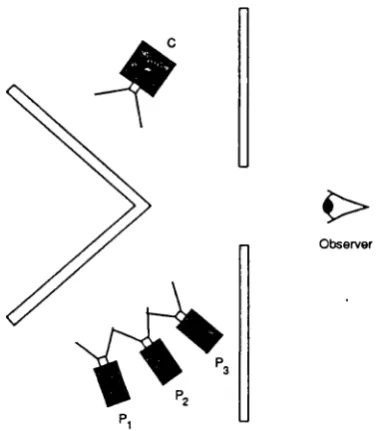
In a color matching experiment, the subject is shown the color to be matched on

one half of the visual field, and a combination of the three primaries on the other.

The observer is allowed to adjust the intensities of the primaries so as to obtain a

color match with the test stimulus, see Figure 1.2. Usually, the color to be matched

has its units normalized to unity in whatever units are being used. It is possible that

the units of one of the primaries may be negative which implies that the particular

primary with a negative intensity should be added to the test stimulus for a color

match with the other two primaries. The color, C, can be a pure spectral color

containing only a single wavelength of light, or it can be a combination of many

different wavelengths. The colors PI, P2 and P3 are the primaries. The coefficients

of these primaries are known as the tristimulus values of the color C relative to the

the primaries used. If the tristimulus values are allowed to take on negative values

then all colors can be matched. Byperforming a color match for all monochromatic

colors, three color matching curves can be created.

1.2.2 Vector Space Methods for Color Representation

If a continuous spectrum is sampled at a sufficient number of points, a vector space

for-mulation of the color matching problem can be obtained [15]. Let the N-dimensional

sampled spectrum be denoted by f = [1(1)

f(2) ... f(N)].

As discussed earlier, the

human visual system has three cone sensors. It can be represented by a matrix,

S = [51 52 53], containing a set of three N-dimensional vectors. The response of the

eye to the spectrum f is then given by:

(18)

Observer

Figure 1.2: Color Matching Experiment

where c is a three-dimensional vector.

Let P

==

[PI P2 P3] denote the N X 3 matrix of primaries where PI, P2 and P3 are

three linearly independent, N-dimensional primaries. Let the monochromatic colors be denoted by ei, i

==

1, ... ,N, where e, has a one in the it h _{component and zeros}

in all others. We say that the stimulus ei is matched by

[mI(i) m2(i) m3(i)]

units of

primaries [PI P2 P3] respectively if

(1.3)

where m,

== [mI(i) m2(i)

m3(i)]T is the three-dimensional vector of the gains of the

pnmaries.

Matching all the spectral colors gives us the equation

(1.4)

(19)

7

chosen to be independent. Both of them are rank three matrices. Therefore the

inverse (STp)-1 exists. Equation (1.4)can be solved for M giving

(1.5)

Post-multiplyingboth sides by P gives us

(1.6)

where I is a 3 X 3 identity matrix.

Using the color matching matrix, M, one can calculate the tristimulus values, tp,

of an arbitrary spectrum according to

(1.7)

where the subscriptP in

t

p denotes the use of the primaries which form the columns of

P. The N-dimensional spectrum, f, is projected onto a three-dimensional subspace

that defines a particular color space. Equation (1.5) relates this subspace to the

human visual subspace. This reduction in dimension can make two different spectra

appear the same to an observer. These spectra are called metamers and the relation

is defined mathematically as

(1.8)

Mathematically, it is not necessary that the primaries P be realizable, i.e. all

elements of P are non-negative. We can choose any set of primaries and obtain the

corresponding matching functions M. Let Q

==

[ql q2 q3] be another set of primaries.

If N is the corresponding set of color matching functions then from Equation (1.4)

we have

ST

==

STpMT

ST

==

STQNT

=? STpMT

==

STQNT

(20)

Post-multiplying both sides of the equation by

Q

and settingNT

Q

to I (from equation

1.6),

we get

(1.10) Substituting back into Equation (1.9), we get

(1.11)

or

(1.12) This transformation also gives us the mapping between the tristimulus values in the two different color spaces

(1.13)

1.2.3 C.I.E.

XYZ

Space

One standard set of primaries is defined by the C.l.E. red, green, and blue primaries consisting of single wavelengths at 700, 546.1 and 435.8 nm. It is seen in Figure 1.3

that the color matching function corresponding to the red primary has negative por-tions in the blue end of the spectrum. This means that the light at these wavelengths cannot be represented by an additive mixture of these three primaries. It is desirable

to have color matching functions which are realizable (i.e. their spectrum contains

only positive or zero values) since the tristimulus values can be obtained by optical filters. The primaries however may be non-realizable which means that they contain one or more negative values in their spectrum and are not physically realizable.

The e.l.E. in 1931 used a 3 x 3 linear transformation to convert the C.l.E. red, green and blue color matching functions to a realizable set of color matching functions

x(,x), Y(A) and z(,x). The transformation from (R,G,B) to (X, Y, Z) is given by:

x

y Z

0.49R

+

O.31G

+

0.2GB

0.1767R

+

O.8124G

+

0.0163B

O.OOR

+

O.OIG

+

O.99B

(21)

9

700 650

500 550 600 Wavelengtl (run) C.I. E. ROBColorMaIcHngFU'ldiona

-,. :-:.--:

__

._--'" I , ,, , , ,, ", , /.. '" ' ~ , , 450 0.2 0.25 0.05 -0.05 0.3

i

0.15 0.1

Figure 1.3: C.I.E RGE Color Matching Functions

700

500 S50 600

Wavelength (nm) C.I.E.xyzColorMatchi'lg FlI'lC'1tons

450 1.8rr--~:----,---_____r--_y__-__r_- _ 14 0." 12 1.6 0.2 06

Figure 1.4: C.I.E XY Z Color Matching Functions

This transformation implied a new set of primaries which were not realizable. Figure

1.4 shows the new set of color matching functions which are non-negative for all

wavelengths in the visible range. The samples are taken every two nanometers but

are connected in the plot. Each of these curves becomes one column of the color

matching matrix, denoted by A. If these columns are now denoted by aI, a2 and

(22)

at regular intervals in the visible range, i.e. at

=

[at(l) al(2) ...al(N)]. Similar

sampling is done to obtain a2 and a3. The tristimulus values can now be computed

in the following manner:

(1.15)

where X, Y, Z denote the three-dimensional components of the tristimulus vector in

this color space.

1.2.4 Urrifor

m

Color

Spaces

The CIE colorimetric system includes computational methods designed to aid in

the prediction of the magnitude of the perceived color difference between two given

object-color stimuli. The determination of a quantity that suitably describes the

color difference an observer may perceive between two given color stimuli rests on

the ability of the observer to judge the relative magnitude of t\VO color differences

possibly perceivable when viewing two pairs of stimuli. The observer's sensitivity

varies greatly with the conditions of observation and the kind of stimuli presented.

Sizes, shapes, luminances, and relative spectral radiant power distributions of the

test stimuli and the stimuli surrounding them are important factors affecting the

observer's judgement.

The eTE recommends the use of two approximately uniform color spaces and

associated color-difference formulae. The recommendations are all given in terms of

the CTE 1931 Standard Colorimetric Observer and Coordinate System [17].

(23)

11

the quantities L*,u* ,v* defined by:

L* 116(

~

)1/3 - 16

Yn

u· 13L·(u'-u~)

13L*(v' - v~) (1.16)

with the constraint that Y/Yn

>

0.01. If values ofY/Yn less than 0.01 occur,

a somewhat modified procedure is recommended for calculating L". For values

of Y/Yn equal to or less than 0.008856, the following L-:n formula is used:

L •m

=

903.3 Y

V

n

Y

for Y

n

~ 0.008856 (1.17)

In Equation (1.16), the quantities u',v' and u~,v~ are calculated from:

u'

=

4X

x

+

15Y

+

3Z V'

=

9Y

x

+

15Y

+

3Z

V'_n

=

(1.18)

The tristirnulus values X n, Yn, Zn are those of the nominally white object-color

stimulus. The total color difference~E:vbetween two color stimuli, each given

in terms of L·, u", V· is calculated from

(1.19)

2. CIE 1976 (L·a*b·)-Space and Color Difference Formula. The second approximately uniform color space, is produced by plotting in rectangular

coordinates the quantities, L*.a",b* defined by:

a*

b*

500[(

-.:£

)1/3 _ (Y)1/3]

Xn Yn

200[( Y )1/3 _

(~)1/3]

(24)

with the constraint that XjXn 1YjYn ,

ztz;

>

0.01. in calculating L"',a* and

b" values ofX/ X n, Y/Yn, Z/Zn

<

0.01 may be includedif the normal formulae are replaced by the following modified formulae

and

L*_m

==

903 3_• _YY

n

Y

for

1: ::;

0.008856

where

a*_m

₌₌

_{500[f(-) -}X f(_o )]Y

X n Yn

b*m

₌₌

200[f(-) -y f(-)]Z

Yn

z;

f(~)

=

7.787(~)+

11166

f(

Y)

=

(Y )1/3

Yn Yn

Y Y 16

f(-)

==

7.787(-)

+

-Yn Yn 116

f(

~)

=

(~)1/3

Zn Zn

Z Z 16

f(

Zn)

=

7.787(Z) +

ill

~

>

0.008856

in

<

0.008856

f.

>

0.008856

f. ::;

0.0088.56

i,.

>

0.008856

i,. ::;

O. 008856 (1.21 )

The tristimulus values _{X n, Yn, Zn are those of}thenominallywhiteobject-color stimulus. The total color difference~E:b between two color stimuli, each given in terms of L

*,

c", b" is calculated from

(25)

13 The CIE color difference measure 6.E:_b is often used as a measure of percep-tual color difference [4, 17]. The average color tolerance accepted in printing applications has been studied and found to be approximately a ~E:b of six. The standard deviation in the accepted tolerance was 3.63 ~E:b [13].

1.3 Thesis

Outline

The thesis is arranged in the following way. The second chapter discusses the mathe-matical formulation of two different color output systems, a CRT and a color printer. The additive principle is discussed followed by the development of a model for a CRT monitor. This is followed by a discussion of the subtractive principle which is used to develop the model for the color printer. The model limitations for both the CRT and printer models are discussed.

The third chapter discusses the calibration procedure for the simulated printer model developed in the second chapter. The ideal model with all its limitations is used to test the calibration method. The bell function and the cubic B-spline interpo-lation techniques that are used are discussed in detail. Three different extrapointerpo-lation techniques, namely, separable linear extrapolation, non-separable linear extrapola-tion and band-limited extrapolaextrapola-tion are discussed. The different interpolaextrapola-tion and extrapolation schemes are compared and the best ones are chosen for the actual printer calibration.

(26)

(SNR) of the printer is calculated and a similar noisy situation is simulated for the mathematical model to see how the model compares to the actual printer. The problem of making sure that all points in the printer gamut can be printed using the look-up table is also discussed.

(27)

Chapter

2 Mathematical Models

Calibration of color output devices such as CRTs and color printers involve data inter-polation techniques. A mathematical model of these output devices which simulates the devices under certain assumptions helps us to study the behaviour of these output devices. The effect of using different interpolation and extrapolation algorithms in the calibration procedure can be studied by applying them to the calibration of the simulated model. This chapter describes the development of mathematical models for a CRT and a color printer. The basic assumptions made in the course of the model development are listed and their validity explained. The basic principles of additive and subtractive color reproduction are also discussed.

2.1 The Additive Principle

(28)

the third primary stimulus can be obtained. Every color stimulus can be matched in color in one of these ways in terms of three primary stimuli whose radiant power can be adjusted by the observer to suitable levels. This is the additive principle. The choice of the three primary stimuli is not entirely arbitrary. Any set that is such that none of the primary stimuli can be color matched by a mixture of the other two may be used. The term additive mixture as used above represents a color stimulus for which the radiant power in any wavelength interval in any part of the spectrum is equal to the the sum of the powers in the same interval of the constituents of the mixture. The additive primaries are represented by three color stimuli in the red, green and blue regions of the spectrum.

The CRT is an output device which is based on the additive principle. In a CRT the image is produced by what is called a picture tube. A picture tube in a color monitor has three electron guns which produce three electron beams which excite three different phosphors (primaries) on a fluorescent screen in front of the guns. The color of the light output depends on the physical properties of the phosphor. The phosphor screen is capable of emitting red, green and blue light. The intensity of the light output depends on the velocity of the beam, the number of electrons in the beam and the type of phosphor used.

2.2 Mathematical Modelling of a CRT

(29)

17

a reasonable assumption in [3, 10]. A non-zero voltage is input to the electron guns

even at a zero code value, i.e. the black portion of the image has a corresponding

non-zero voltage level. For a black and white monitor, which has only a single electron

gun the mathematical relationship making use of the above assumption is given by:

L

==

K(n - xo)'"Y (2.1)

where L is the radiance of a black and white phosphor, K is a constant dependent

on the units of L, n is the count value in the frame buffer, and Xois the cutoff count

value for the electron gun.

For a color monitor, the model takes a more complicated form. If we assume that

the chromaticity coordinates of the three phosphors remain constant then we get the

following equation:

K1,R(R - Ro)'YR

+

K1,a(G - Go)'"YG

+

K1,B(B - BO)'YB K2,R(R- Ro)'"YR

+

K2,G(G- Go)'"YG

+

K2,B(B - BO)'"YB

K3,R(R - Ro)'"YR

+

K3,G(G - Go)'"YG

+

K3,B(B - BO)'"YB (2.2)

where LR ,La, LB are the radiance values for red, green and blue phosphors, R, G, B

are the red, green and blue count values, Ro, Go, Boare the red, green and blue cutoff

count values, and ,R"a"B are the exponents for thee red, green and blue electron

guns. The terms Ki,R' Ki,G, Ki,B, i

==

1,2,3 are constants. If the condition for gun

independence is met, then Equation (2.2) can be further simplified as:

K1,R(R -

Ro)'"YR K2,a(G- Go)'"YG

K3,B(B - BO)'"YB (2.3)

(30)

2.3 Limitations of the CRT Model

A color monitor has four important properties which are assumed in developing a

mathematical model

[3, 10].

These assumptions are true to varying degrees. They

are:

1. Temporal Stability: The monitor maintains its colorimetric parameters over time, so that a calibration is not necessary frequently. In practice, this is true

over days but usually monitors should be calibrated about once a month.

2. Spatial Uniformity: The monitor has the same colorimetric parameters at different points on its screen, so that a calibration can be done at one place

on the screen that will hold for the whole screen. Spatial uniformity is hard to

achieve. Sometimes there is as much as a 50 percent variation in the luminance

value between the color displayed at the center of the screen and the same color

displayed at the corners. This is due to the improper focusing of the electron

guns at the corners of the screen and the fact that electrons must travel a

longer distance to illuminate the screen corners compared to the center.

3. Gun Independence: The colorimetric properties of the monitor are truly

additive, so that it is possible to base the calibration scheme on the assumption

that the displayed color is the additive mixture of the color produced by each

of the three phosphor gun combinations. This property is assumed to hold in

most monitors.

4. Phosphor Constancy: The chromaticity coordinates of the red, green and blue phosphors remain constant independent of the voltages applied to the

electron guns. Mathematically, if the spectral distribution of the phosphor is

(31)

19

voltage

V2

is given by

<P2(A)

=

a<pl(A)

for some constant a. This property is

also assumed to hold in most monitors.

2.4 The Subtractive Principle

In additive methods of color reproduction, all colors are produced by the adding

together of different proportions of the light from three primary colors, a red, a green,

and a blue. Subtractive color reproduction is different in the sense that all the colors

are produced by different proportions of three different colorants, cyan, magenta and

yellow. It is characterized by the property that color is obtained by removing selected

portions of a source spectrum (Figure 2.1).

~ ~

-

-Red Red Red Red

ro ~

CD C +oJ

~ Q)

."t:: (Tj

Green c Green Green (/)

.c Green ~ Q) 0 ::J

~

o

C'> Q) ~

eu

_>-

_Ci

~

Blue Blue Blue

Blue

-

~

-

-Figure 2.1: Subtractive Model

A printing process is subtractive in nature. Each of the cyan, magenta and yellow

colorants removes an amount of its complimentary color. The function of the cyan

colorant is to absorb red light, that of the magenta colorant to absorb green light,

and that of the yellow colorant to absorb blue light. The transmission curves of each

of the three colorants vary over the entire spectrum as shown in Figure 2.2. The

amount of a particular color removed is related to the concentration of the colorant.

(32)

GO 80 70 (a) ~ ... I ... , .' ....

," /..r>; "" .... ,

I

I / .,.1 .... , ' , ,

,". \

"

...;' " -. ,

"/:/

\'... ",

30 I . ' "

" .::;, "'<:

(C;,

,(b)

20 :'i '. ". ,

.... i (d),.,.""... "" -. ""

10'/ - . " '_, _'_...

.....

_---~o ~ ~ ~ ~

WaV'efeog1h (rvn)

TranwtuWooCuvestOfDt1'fenr(Concenntlonsof Magenta Dye

700 so 80 700 ,.--' 650

• . _- ' - 0 , 1 '

....

-500 550 600

Wavefeogth (rvn)

~O

~o ~ ~ ~ ~ 700

Wav_8fl91h (rvn)

Tranarrissloneurv.sfofOdferentConcentralOOSofYellowDye (a)

" "

(bY" . /~/...

,~ (~., /

, . : . '

, : . ' (<1)

"

,'." "

, .... "

I : ,.

"

....: , /

I .: "

" .::./ ,,,.::".' ... -:,. 70 , , ~ , ' . .

J : . '

_~) J .: . '

, ....

"

.../

" " I : . , .

, ..•.~c) \ " :.... , / 30 .... ... "

. (d)' " .'

20

-<./-

,.,.~

""

" ,.'

" ... '

:.,.

, -, ,,,J.,/~/

....~..~-~..-.~.~..~.:~/ 10 ~ 100 so 80 70 S 60 1 ~ ₅₀ = t= ~ 40 30 20

10 ,_....

... 0 ' " , ~...-.

(33)

22

transmission with concentration is not large but, in the bluish part of the spectrum, the transmission depends very markedly on the concentration of the colorant. This shows that the amount of bluish light reflected from a piece of white paper, viewed in daylight, would be altered by the concentration of a yellow colorant on its surface. Similarly, the main effect of altering the magenta colorant is to vary the transmission in the greenish part of the spectrum, while altering the bluish and reddish parts to a smaller extent. Different concentrations of the cyan colorant alter the transmission in the reddish portion of the spectrum and to a lesser extent the transmissions in the greenish and reddish parts of the spectrum.

2.5 The Forward Model

of

the

Printer

Each of the colorants can be characterized by their optical density spectra, the N x 3 matrix D. The optical density of a colorant is defined as -loglo(T), where T

represents the transmittance or reflectance of the colorant. The density of a colorant is proportional to its concentration c. Thus we can write [7]

i

==

1,2,3

(2.4)

where c; is the concentration of colorant i and Di,max is the density at unit

concentra-tion for colorant i. Transmission of a particular colorant, T; is related logarithmically to its density as

i == 1,2,3

(2.5)

If we look at the density spectra for the different colorants, we see that the curves should be linear in density, i.e. Di(Ci,l

+

Ci,2)

==

Di(Ci,l)

+

Di (Ci,2) for different

concen-trations £;,1 and £;,2 of a particular colorant i. This can be seen in Figure 2.3. The

observed spectrum at a particular wavelength ,\ is given as [16]

(34)

23

where Ti ( '\ ) is the transmission of the it h colorant at wavelength ,\ and 1('\) is the

intensity of the illurninant at wavelength X, This is the case for the colorants being placed upon film. In the case where paper is used, the paper reflects the light and the light passes through each layer of the colorant twice. Substituting Equation (2.5) into Equation (2.6) we get:

(2.7)

Thus, the forward model can be written algebraically as

[16]

(2.8)

where c is the 3-vector representing the concentration of the colorants, Dm a x is an

N

x

3 matrix of the densities at the maximum concentration, L is an N

x

N diagonal matrix of the illuminant spectrum and g is the N-vector representing the radiant spectrum. The concentration values must be between zero and unity. The exponential term is computed componentwise i.e.

(2.9)

This model ignores non-linear interactions between colorant layers. The tristimulus values XY Z are obtained by the equation

(2.10)

where A is a N x 3 matrix of the CIE color matching functions.

2.6 Limitations of the Printer Model

(35)

24

1. Temporal Stability: The amount of colorant that is printed onto the pa-per (for a particular control vector) remains the same each time it is printed. Therefore the colorimetric parameters do not change over time so that calibra-tion needs to be done only once.

2. Spatial Uniformity: The printer behaves identically over different regions of the printer sheet. The amount of colorant laid down on the sheet does not depend on its spatial location on the sheet. In the case with printers which have different printer heads, this implies that each of these heads are identical in nature and there is no variation in the amount of colorant put down due to variation of these heads. This would imply that the calibration can be done for all the heads simultaneously.

3. Ideal Transmissions and Reflections: This is one of the most important assumptions of the mathematical model. We assume that the paper reflects all the light which is incident onto its surface without any absorptions. This is followed by ideal absorptions and transmissions by each of the colorants. We assume that there are no first-surface reflections at a dye surface when light is incident on it, see Figure 2.5. We also assume that there are no multiple internal reflections and \ve model the path that is indicated in Figure 2.5.

4. No Interaction Between Colorant Layers: A dye laid down on top of another dye does not adhere as well as it would to paper. This is called dye inhibition which we assume is absent in the model. In a thermal dye transfer printer, the heating for a subsequent dye can melt the dye that has been previously laid down. This is called back-transfer which we assume is absent in this model.

5. Spectral Characteristics of Dye are not Changed by Interaction: We

(36)

spectral characteristics of each of the individual dyes.

The above properties represent an ideal printer. However, in reality, a printer may behave quite differently. The assumption of having identical printing heads may not be a reasonable assumption as was the case with the printer that was calibrated in the course of this work. Each of the printer heads show a certain amount of variability. This would imply different calibrations i.e. look-up tables, for each of the heads.

Incident Light

A

Observer

Paper

Figure 2.4: Scattering of Light

(37)

26

path we are modelling

Paper

First Surface Reflection

Paper

Multiple InternaJ Reflections

Figure 2.5: Other Paths of Light

reflection of the incident light at the surface of the dye. Multiple internal reflections occur when some of the light reflected by the paper is reflected back toward the paper by the upper surface of the colorant, passing through the colorant to be reflected again by the paper. Eventually it either emerges or is absorbed.

(38)

Chapter

3 Mathematical Formulation

This chapter deals with the detailed description of the calibration procedure per-formed for a simulated printer. The mathematical model developed in the second chapter is used in the simulation. The calibration of this simulated printer will help us understand and study some of the problems encountered in the actual calibration of a printer which is described in the next chapter. This chapter describes in detail the different interpolation and extrapolation techniques that are used in the calibration. These schemes are then implemented with the mathematical model and the results compared so that the best schemes can be chosen for the actual printer calibration which is discussed in the next chapter.

3.1 Interpolation Technique

Using the mathematical model developed in Chapter 2, a coarse 8 x 8 x 8 look-up table mapping the control values to the output eTE L*a*b* values is generated with the forward model of Equation (2.8). This forward model is used for testing only and to help us predict how well each of the the interpolation functions that we use, will perform for the actual printer calibration. We have from the forward model

(39)

28

where c is a 3-vector of control values and t is a 3-vector of the eIE L*a*b* values. The function F here refers to the interpolation function that is used to define this mapping. The forward model is shown in Figure 3.1.

-Control Values

t

=

F(c)

Color Space

Figure 3.1: 'I'he Forward Model

The mapping from the control value space to the CIE L*a*b* space is highly non linear. Our problem now consists of creating a finer, regular grid in the CIE L*a*b*

space, such that each point on this fine grid in the color space has a known control vector associated with it, i.e. for a certain

CIE

L*a*b* vector

t

g on this finer regular

grid the corresponding control vector c_g is obtained. Since the forward mapping is not defined for the actual printer, we make the same assumption with the mathematical model and define the interpolation function as an approximation to the function F. A fixed set of data points (8 X 8 x 8) are used taking into account the fact that it is

convenient to take only a small number of measurements from the printer.

Iterative techniques with interpolation are used to estimate the control vector corresponding to every vector tg on the finer grid in the CIE L*a*b* space. The

mapping from the control value space to the Clf

L*a*b*

space is not given by an

(40)

us use a fixed point iteration. For a given ClE L*a*b* vector

t

g , an initial estimate Co of the control vector is made and the corresponding CIE L*a*b* vector is obtained

by interpolating over the three-dimensional regular grid of control values. A special form of Newton's method in three dimensions is used to obtain a new estimate of the control value. This method is called Broyden's method [5] and is equivalent to finding a root of the equation

F(

c) ==

t

g or F(

c) -

t

g

==

0 (3.2)

where the function F refers to the interpolation function that is used. This iteration is continued until Equation (3.2) is solved to the selected degree of accuracy. Broyden's method is described in Appendix A.

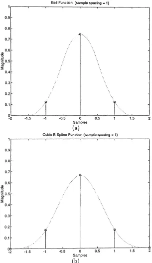
Two kinds of interpolation functions were used, the bell function and the cubic B-spline function. They are described below:

1.

Bell function:

This function is obtained by the convolution of a triangle function with a square function and is defined as

[12]

The sample spacing is assumed to be unity.

-3

<

x

<

-1

2 - - 2

.=.!<x<!

2 - - 2

!<x<~_{2 -} _- ₂

(3.3)

2.

Cubic B-spline function:

This function is obtained by the convolution of the bell function with a square function. It is defined as

[12]

(3.4)

(41)

30

BeU Function (sample spacing - 1)

0.9 0.8 0.7 0.6 ~ .a 'c0.5 0) t1J ::E 0.4 0.3 0.2 0.1 0

-2 -1.5 -1 -0.5 0 0.5

Samples

(a)

Cubic S-Spline Function (sample spacing • 1)

1.5 2 0.9 0.8 0.7 0.6 ~ .2 C 0.5' 0) t1J ~ 0.4 0.3 0.2 0.1

-2 -1.5 -1 -0.5 0 0.5

Samples

(b)

1.5 2

(42)

Three-dimensional separable interpolation is used to interpolate for the CIE L*a*b* values tg

=

(tg,l' tg,2,tg,3)on the finer grid

L L L

w/(i,j, k)S(Cl,p - i)S(C2,q - j)S(C3,r - k)

k j i

p,q,i == 1, ... ,8 I == 1,2,3 (3.5)

where Wl(i, j,k) are the weights used to interpolate, S denotes the interpolation func-tion used and (CI, C2, C3) denotes the control vector. The weights Wl(i, j,k) are ob-tained by solving three sets of linear equations, one for each 1, as shown above. The values tg,l(Cl,i, C2,j, C3,k) are assumed to be equal to the value of the ijkt h scalar entry in the given set of data points tg,I(Cl,i, C2,j, C3,k), for i,j,k == 1,2, ... 8 and 1

==

1,2,3.

3.2 Extrapolation

(43)

32

extrapolation. The last scheme was investigated since the mapping from the CMY colorants to the CIE L*a*b* space for a printer is usually well behaved and smoothly varying.

. .

. . . . .

. . .

.

. . . .

.

. . .

.

....,-..t-..•..

-t..-t , ' ,-..'-

.

....

'-

..: : : : : : : :

'-

.

...

...~ .

...

...~ .

..··t··

..·t···

....+-..

...~

....

....t..

·..

t·..·

...

...+. .

....'-..

_{. . . .}

.

_.

. .

...J.. .

".-...'-..

~

..

~

..-t...

t-..,...

+-..•..•....

i

~

;

~

; ; ; ; ; i

Control value space

• Points to be Extrapolated

Figure 3.3: Extrapolation in the Control Value Space

3.3 Extrapolation Methods

The

eIE

L*a*b* components are each assumed to be separable functions ofthecontrol values of cyan, magenta and yellow, i.e. we can write

a* == 9 (C1 , C2, C3) ==91(C1) 92(C2) 93(C3 )

b" = h(Cl'C2, C3) == h1(Cl) h

2(C2)

h

3(C3)

(3.6)

(3.7)

(3.8)

Since we assume separability, the separable extrapolation schemes were implemented

in a one-dimension problem to compare the relative errors that occur in the

(44)

33

were created by keeping two of the colorants constant and varying the third. The

true L· values corresponding to these control values are then compared with the

orig-inal L* values to calculate the error. Two different separable extrapolation schemes

were used, linear extrapolation and band-limited extrapolation. These methods are

discussed in detail in the following subsections. The third method of non-separable

linear extrapolation is also discussed.

3.3.1 Separable Linear Extrapolation

Linear extrapolation is the simpler extrapolation of the t\VO and is carried out one

dimension at a time. The extrapolations were carried out along each of the colorants,

one at a time. The order, cyan, magenta and yellow was selected. Let

ti,

i = 1, ... 8 be

the set of eight data points representing the L* values which correspond to different

concentrations of cyan in the range (0,1) and zero concentrations of magenta and

yellow. The extrapolated points,

to

and

t

g , corresponding to concentrations of -1/7

and 8/7 of cyan respectively, for the same concentrations of magenta and yellow are

obtained by simple linear extrapolation as follows:

(3.9)

Similarly,

(3.10)

In this manner, all the extrapolations are done along the cyan direction for

dif-ferent concentrations of magenta and yellow. These extrapolated points are now

included in the data set to perform extrapolations in the directions of each of the

other colorants. This then involves taking a set of eight data points for which the

concentrations of cyan and yellow are kept constant and magenta is allowed to vary

(45)

34

are now included in the data set and extrapolations are carried out in the yellow di-rection by selecting eight data points with constant cyan and magenta concentrations but different concentrations of yellow in the range (0,1).

The same procedure as above is followed for the data points corresponding to the a* and b" values. This gives us the final set of extrapolated data. In this process, the 8

x

8

x

8 grid is now augmented to a 10

x

10

x

10 grid. All these data points can now be used in the interpolation algorithm.

3.3.2 Linear Extrapolation using Taylor Series Expansion

This method of linear extrapolation performs a non-separable vector extrapolation. If Co is a measured control value point on the boundary of the control value space of

the printer then let the corresponding point in the eIE L*a*b* space, to, be denoted by F(co). Using the Taylor series expansion we can make a linear approximation for any point c, not in the control value space in the following manner:

(3.11)

where A is a 3 x 3 matrix and has the following form:

8L 8L 8L

aco1 8co2 8t:{)3

A== _aCO.lad. _8CO.2ad. _{8co 3}ad (3.12)

8b 8b ab

aCO,l 8CO,2 8CO,3

A can be approximated by using least-squares. We first estimate A by using the points neighbouring the boundary point Co of concern. Each of these points forms

(46)

neighbours. This results in three sets of simultaneous equations with eleven equations

each. A least-squares approach is used again to solve for A. Finally, a point lying on

one of the faces of the gamut, is surrounded by seventeen neighbours. This involves

solving three sets of simultaneous equations with seventeen equations each. Again,

each set of equations solves for each row of the matrix A. Once A is known, we

can easily approximate F(Ci) for any c, just outside the printer range using Equation

(3.11). This gives us a set of extrapolated data. Using this extrapolation method

our 8 X 8 X 8 data set is augmented to a 10 X 10 X 10 data set. All these points can

then be used in the interpolation algorithm to build the finer, regular grid in the CIE

L*a*b* space.

3.3.3 Band-Limited Extrapolation

A well-known technique for solving the extrapolation problem is an iterative method

known as the Papoulis-Gerchberg algorithm. Before we discuss this algorithm, let us

state the band-limited extrapolation problem for a discrete periodic sequence. For a

one-dimensional problem, let

g(

m), m E Z be a discrete periodic sequence with a

period N

==

2M

+

1 (without any loss of generality) such that

g{m)=g{m+N) mEZ

Assume also that 9 is band-limited to

[-ko, ko],

so that

N-I

L

g(m)e21rirnk/N

=

0 if

M::::

Ikl

>

k

o

m=O

(3.13)

(3.14)

If we are given a piece of 9: g(m), m E [-L, L], our goal is to recoverg(m), m

rt

[-L, L]. We can now state the discrete-discrete band-limited extrapolation problem

asfollows:

(47)

36

find f(m), -M::; m ~ M, M

>

L, such that

f(m)

==

g(m), m E [-L,L];

f

is band-limited to _{[-ko, ko].}

An iterative extrapolation technique is discussed by Papoulis in

[11].

However, this technique has to be modified when only sampled data is available [6]. A possible technique of implementing the iterative technique is by means of the DFT. The first iteration is given with the DFT

M

G(m)

==

L:

g(j)e-21rijm/N

j=-M

The nth iteration step proceeds as follows. We form the function

where

(m) _

{I

I

m

I

<

ko

p - 0

Iml

>

k_o

(3.15)

(3.16)

(3.17)

This is equivalent to band-limiting Gn - 1 to the band-limit of

f.

We then compute

the inverse DFT of E: as below:

We next form the function

. {g

(j ) Ij I~ L

gn(J)

=

fn(j)

Ijl

>

L

(3.18)

(3.19)

obtained by replacing the segment of

fn(j)

in the interval [-L, L] by the known segment

g(j)

of

f(j).

The nth step ends by computing the transform

M

Gn(m)

=

I.:

gn(j)e-27riim/N

j=-M

(48)

of the function

9n(j)

so formed. The iteration is carried out until the selected degree of accuracy is achieved i.e. until 9n ~9n+t.

The method described above is used to extrapolate the data that we have. One-dimensional band-limited extrapolation is carried out, one dimension at a time. As in the case of separable linear extrapolation, the extrapolation are done first in the cyan direction, i.e. the concentrations of magenta and yellow are kept constant while those of cyan are allowed to vary. This is followed by extrapolations in the magenta and yellow directions.

To compare the separable linear and band-limited extrapolation schemes, a series of lines of the luminance (L*) values are chosen by keeping two of the dyes constant and varying the third. Each of these lines consists of eight points (by varying one of the dyes from 0 to 1 in steps of 1/7, and keeping the concentrations of the other two dyes constant). Extrapolations are carried out for one point on either side to give us a set of ten points. These ten points are then used in an interpolation routine to estimate the control value for different values of the luminance which lie within the range of the original eight data points. Figure 3.4 shows a typical comparison of interpolation errors using points generated by both these extrapolation schemes.

(49)

38

Error forLCurve

0.25

02

g

0.15 w

0.1

0.05

- usJnglinearextrapolation

_ usingband-limitedextrapolation

Cone ofmagenta -0.5714

Cone of yeHow - 0.5714

0.1 02 0.3 0.4 0.5 0.6 0.7 0.8 0.9 Concentration of Cyan

Figure 3.4: Errors due to Different Extrapolation Methods

3.4 Interpolation Methods

The points obtained by linear extrapolation are then used along with the data points

from the mathematical model to create a finer, regular LUT in the CIEL*a*b* space.

The bell and spline interpolations functions described in section 3.2 are used in the

interpolation routine to create the grid. A simple algorithm was used to divide the

CIE L*a"b" space into an equi-spaced grid. A minimum grid size of 32 was used in

each direction. The spacing in the grid was calculated in the following manner

• Divide the range in each of the L*.a" and b* directions (obtained from the 8 X

8 X8 LUT) by the minimum grid size i.e. form the spacings

(L':nax - L':nin)/31,

(a~ax

-

a~in)/31 and (b~ax

- b':nin)/31.

• Choose the minimum of the spacings formed above as the spacing between the

(50)

This algorithm gives us a regularly spaced grid such that the spacing in each of the

L

*,

a* and

t:

directions is the same.

Each of the CIEL*a*b" points on this regular grid are fed through the interpolation

routine to obtain a corresponding control vector. The ~E errors for each of these points can be easily calculated since the mathematical model gives us the 'true' CIE

L*a*b*value corresponding to the control vector which is obtainedbythe interpolation routine. In the case of the actual printer, this would correspond to the actual color that the printer prints on the paper as opposed to the color it is supposed to print.

The bell and spline interpolation functions perform almost identically for the mathematical model. Figure 3.5 and 3.6 show the histograms of the ~E errors for each of the two cases. The histogram includes all the points which have converged to control vectors which lie within the range of the printer i.e. each of the control values lie in the range (0,1). It can be seen from the two figures that the bell function shows a smaller average 6.E error. As a result, the bell function was the interpolation function chosen for the actual printer calibration which is discussed in the next chapter.

(51)

mean-Q.417g

varianee-O .1130

IIof points in gamut-18164

,... ... ...

~

Histogram of dE Errors for the Points on the Regular Grid (32x40x52) 2000 1800 1600 1400 1200 ~ c ~1000 ~ Lt 800 600 400 200 o

o 02 0.4 0.6 0.8 1

dE

1.2 1.4 1.6 1.8 2

40

Figure 3.5: LlE Errors Using Bell Interpolation

Histogram of dE Errors for the Points on the Regular Grid (32x40x52)

mean-Q.4292

variance-Q.0995

II of pointsin gamu1-18165

,...

-rtnrrnrh~

2000 1800 1600 1400 1200 ~ c ~1000 e u, 800 600 400 200 o _o

02 0.4 0.6 0.8 1

dE

1.2 1.4 1.6 1.8 2

(52)

Histogram of dE Errors for Mathematical Model 3500 3000 2500 (j' c ~2000 e u.. 1500

mean - 1.2648

variance - 2.7275

IIof points in gamlA - 31234 dE >2 - 6343points

6 8 10

dE

12 14 16 18 20

Figure 3.7: ~E Errors Using Bell Interpolation & Separable Linear Extrapolation (Includes Out-of-Gamut Points)

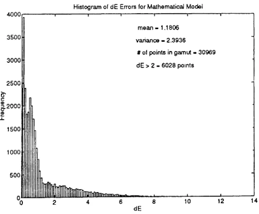
Histoqram of dE Errors for MathematicaJ Model

mean - 1.1806

variance - 2.3936

#of points in gamut - 30969 dE > 2 - 6028 points 4000 3500 3000 2500I (j' c ~2000 (Z) u: 1500 1000 500 0 2

0 4 6

dE

8 10 12 14

(53)

42

3.5 Signal-to-Noise Ratio Description

The results obtained in the previous section describe the performance of the interpo-lation routine under the assumption that no noise is present in the data collection. However, in reality, a color printer will not be noise free and the noise will manifest itself as a positive or negative variation about the true value of the data that is col-lected. The primary causes are the variability of the printer, the interactions between the colorant layers and the variability in the measuring device.

To simulate this environment, noise is added to the data from the mathematical model and its effect on the change in ~E errors is observed. The noise is added in the XY Z tristimulus space. The XY Z values of the data points are generated from the mathematical model as described in Chapter 2. If Xi, i

==

1, ... , 512 is the set

of data points without the noise then the signal power is calculated in the following manner:

512

2 " 2

O'signal

==

Z::Xi

i=l

(3.21 )

The noise power depends on the SNR (in db) that is desired and is calculated in the following manner:

2 2 -SNR

U noise

==

0'signal10 10 (3.22)

(54)

(55)

45

The basic thermal dye transfer process consists of transferring the dye which is on a carrier ribbon to another substrate, paper or transparency

[14].

The ribbon is made with successive strips of yellow, magenta and cyan dyes. The yellow image is laid down first; the paper is repositioned; the magenta image is then laid down; the paper is repositioned and the final cyan image is laid down. The paper and ribbon are moved simultaneously over a thermal head which melts or vaporizes the dye and thus transfers it to the paper (Figure 4.1). The printing head consists of one individually controlled heating element for each pixel on a line. This allows the thermal printers to produce high resolution images. The XL 7700 head contains 2048 individual heating elements. Thermal control of each element drives the appropriate amount of dye from the ribbon onto the paper or transparency material, thus forming a continuous tone picture.

Printer Ribbon

Paper or Transparency

Print Head

Drum

(56)

A number of problems can a.rise with the thermal dye transfer methods. These include:

• variability of the heating elements

• variable warm-up time and behaviour of the heads

• variation caused by ambient conditions

• hysteresis of the heating elements

• dye inhibition, a dye laid down on top of another dye does not adhere as well as it would to paper

• back transfer - the heating for a subsequent dye can melt the dye that has been previously laid down

In addition to these errors, errors are also introduced due to the calibration method that is used. These errors will mainly be errors due to measurements and interpola-tion schemes that are used. All these errors will be discussed in greater detail with reference to the calibration of the XL7700.

4.2 Data Collection and Observations

A calibration chart was generated from the the Kodak XL7700 by varying the con-centrations of the cyan, magenta and yellow dyes in a uniform manner. The control value space was divided into eight equispaced samples in each direction (from 0 to 1in steps of 1/7) to generate 512 color patches. A GRETAG SPM-50 spectrophotometer was used to measure the

eIE

L*a*b* values of these color patches. This set of

eIE

L*a*b* values forms the known coarse 8

x

8

x

8 data set.

(57)

47

proceeding further with the calibration process, it was important to determine if there were any variations in the printouts produced by the XL 7700. Different factors contribute to the error during the calibration process of the printer. These errors appear at every stage of the process. One of the important contributions to this error is the inherent variability of the printer. Four kinds of inconsistencies were observed due to the printer variation. These variations of the printer were used to give us an estimate of the noise for the SNR calculation of the printer.

Printer Calibration Procedure

Calibration Chart

CIE L*a*b* Image

CIE L*a*b* to CMY Look-Up

Table

Printer

Figure 4.2: Processing the Image for Printing

1.

Initial

Warrn- Up Time:

The XL7700 has an initial warm-up time.

Several identical images of the calibration chart were printed out in succession as soon as the printer was ready for printing. However, after measurements of the first two charts were made, it was noticed that there was an appreciable color difference between the CIE L*a"b' values of the color patches on the first

(58)

48

more were observed between the first print and the second print. However, when successive prints were compared with these two initial prints they were much closer to the the second print than the first. _~E errors of the order of 10 were still observed between each of these prints and the first. It was concluded that the first print produced by the XL 7700 after it is switched on is an inaccurate representation of the true image. An initial print was the warm-up time assumed for the printer for all future measurements i.e. only the prints after the first were used in the calibration process.

2.

Measurernents on Different Heads:

The CIE L*a*b* values

pro-duced by identical control values varied depending on the position of the color patch on the paper on which it was printed. Preliminary data collected on several patches (corresponding to the same control value) printed at different positions on the sheet typically gave ~E errors greater than 3.5. Since the XL 7700 has four heads printing over different areas of the paper, a natural explanation for the error was that the amount of dye printed on to the paper was also a function of the particular head that printed it. This led to the conclusion that the calibration should be carried out for each individual head. In the calibration procedure used, the calibration chart was printed only under the second head.

3.

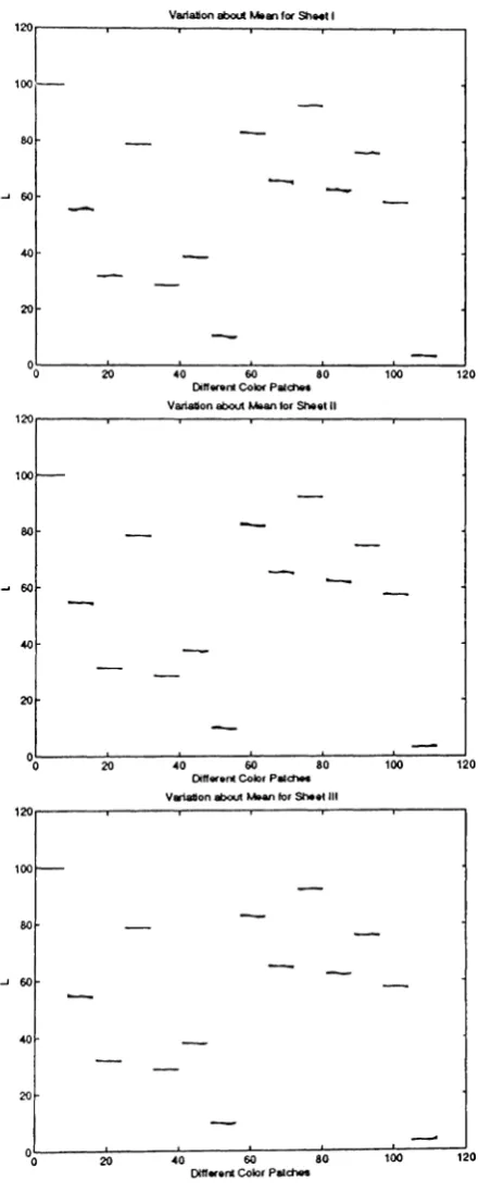
Measurernerrts on Different Sheets of Paper:

The XL7700

(59)

49

measurements of the calibration chart were measured over several printouts and the average values over all the sheets were used as the points of the known 8 x 8x 8 coarse data set. Another problem arose at this stage since the entire calibration chart (which consisted of 512 color patches) could not be printed on one sheet under the second head only. Each color patch had to be large enough for it to lie completely under the aperture of the GRETAG SPM-50 spectrophotometer. This meant that the calibration chart had to be printed on two separate sheets, each sheet containing half the total number of color patches on the chart. Since all the color patches were generated sequentially by changing the concentration of the cyan, magenta and yellow dyes successively in that order, it was obvious that the measured errors would incur a block change when half of the chart was printed on a new sheet. Therefore, larger errors would occur in the regions where adjacent color patches of the calibration chart were printed on different sheets. To keep this error random and not just in one region of the CIE L*a*b* space, the calibration chart was printed out in a random manner. These measurements were then averaged over several printouts to obtain average CIE L*a*b* values for all the 512 points of the coarse LUT. Figure 4.3 shows the calibration chart which was printed out in an ordered fashion under the second head.

4.

Error due to the Measuring Device:

Another source of error is

(60)

Interpolation and extrapolation in color systems