Miniaturized embedded stereo vision system (MESVS)

Scholarship at UWindsor

Scholarship at UWindsor

Electronic Theses and Dissertations Theses, Dissertations, and Major Papers

2008

Miniaturized embedded stereo vision system (MESVS)

Miniaturized embedded stereo vision system (MESVS)

Bahador Khaleghi University of Windsor

Follow this and additional works at: https://scholar.uwindsor.ca/etd

Recommended Citation Recommended Citation

Khaleghi, Bahador, "Miniaturized embedded stereo vision system (MESVS)" (2008). Electronic Theses and Dissertations. 7870.

https://scholar.uwindsor.ca/etd/7870

This online database contains the full-text of PhD dissertations and Masters’ theses of University of Windsor students from 1954 forward. These documents are made available for personal study and research purposes only, in accordance with the Canadian Copyright Act and the Creative Commons license—CC BY-NC-ND (Attribution, Non-Commercial, No Derivative Works). Under this license, works must always be attributed to the copyright holder (original author), cannot be used for any commercial purposes, and may not be altered. Any other use would require the permission of the copyright holder. Students may inquire about withdrawing their dissertation and/or thesis from this database. For additional inquiries, please contact the repository administrator via email

(MESVS)

by

Bahador Khaleghi

A Thesis

Submitted to the Faculty of Graduate Studies through the

Department of Electrical and Computer Engineering in Partial Fulfillment

of the Requirements for the Degree of Master of Science at the

University of Windsor

1*1

Published Heritage Branch

395 Wellington Street OttawaONK1A0N4 Canada

Direction du

Patrimoine de I'edition

395, rue Wellington OttawaONK1A0N4 Canada

Your file Votre r&terence ISBN: 978-0-494-57616-8 Our file Notre reference ISBN: 978-0-494-57616-8

NOTICE: AVIS:

The author has granted a

non-exclusive license allowing Library and Archives Canada to reproduce,

publish, archive, preserve, conserve, communicate to the public by

telecommunication or on the Internet, loan, distribute and sell theses

worldwide, for commercial or non-commercial purposes, in microform, paper, electronic and/or any other formats.

L'auteur a accorde une licence non exclusive permettant a la Bibliotheque et Archives Canada de reproduire, publier, archiver, sauvegarder, conserver, transmettre au public par telecommunication ou par I'lnternet, preter, distribuer et vendre des theses partout dans le monde, a des fins commerciales ou autres, sur support microforme, papier, electronique et/ou autres formats.

The author retains copyright ownership and moral rights in this thesis. Neither the thesis nor substantial extracts from it may be printed or otherwise reproduced without the author's permission.

L'auteur conserve la propriete du droit d'auteur et des droits moraux qui protege cette these. Ni la these ni des extraits substantiels de celle-ci ne doivent etre imprimes ou autrement

reproduits sans son autorisation.

In compliance with the Canadian Privacy Act some supporting forms may have been removed from this thesis.

Conformement a la loi canadienne sur la protection de la vie privee, quelques

formulaires secondaires ont ete enleves de cette these.

While these forms may be included in the document page count, their removal does not represent any loss of content from the thesis.

Bien que ces formulaires aient inclus dans la pagination, il n'y aura aucun contenu manquant.

Publications

0.1 Co-Authorship Declaration

I hereby declare that this thesis incorporates material that is result of joint research, as follows:

This thesis also incorporates the outcome of a joint research undertaken in collaboration with Mr. Siddhant Ahuja under the supervision of Professor Jonathan Wu. The collabora-tion is covered in Chapter 4 of the thesis as the design and development of the hardware for this work has been done by Mr. Siddhant Ahuja. In all rest of the cases, the key ideas, primary contributions, experimental designs, data analysis and interpretation, were performed by the author, and the contribution of co-authors was primarily through helping in obtaining experimental results presented in section 5.2 and also providing some of the ideas presented in section 4.3.3.

I am aware of the University of Windsor Senate Policy on Authorship and I certify that I have properly acknowledged the contribution of other researchers to my thesis, and have obtained written permission from each of the co-author(s) to include the above material(s) in my thesis.

0.2 Declaration of Previous Publication

This thesis borrows some of its material from two original papers that have been previously published, as follows:

1. B. Khaleghi, S. Ahuja, and Q. M. Jonathan Wu, "A New Miniaturized Embedded Stereo-Vision System (MESVS-I)", CRV 2008 (to appear).

2. B. Khaleghi, S. Ahuja, and Q. M. Jonathan Wu, "An Improved Real-Time Minia-turized Embedded Stereo-Vision System (MESVS-II)", IEEE CVPR Workshop on Embedded Computer Vision 2008 (to appear).

I certify that I have obtained a written permission from the copyright owner (s) to include the above published material(s) in my thesis. I certify that the above material describes work completed during my registration as graduate student at the University of Windsor.

Stereo vision is one of the fundamental problems of computer vision. It is also one of the oldest and heavily investigated areas of 3D vision. Recent advances of stereo match-ing methodologies and availability of high performance and efficient algorithms along with availability of fast and affordable hardware technology, have allowed researchers to develop several stereo vision systems capable of operating at real-time. Although a multitude of such systems exist in the literature, the majority of them concentrates only on raw perfor-mance and quality rather than factors such as dimension, and power requirement, which are of significant importance in the embedded settings.

Declaration of Co-Authorship/Previous Publications iv

0.1 Co-Authorship Declaration iv 0.2 Declaration of Previous Publication v

Abstract vi

Acknowledgements vii

List of Figures xi

List of Tables xiv

1 Introduction 1

1.1 Problem Statement 1

1.2 Motivation 2 1.3 Thesis Organization 3

2 Stereo Vision Literature 6

2.1 Stereo Vision 6 2.1.1 Taxonomy of dense stereo matching methodologies 7

2.1.2 Challenges 8 2.1.3 Constraints and Assumptions 10

2.2 Stereo Matching Methodologies 13

2.2.3 Local vs. Global 18 2.2.4 State of the Art 21

3 Real-time Stereo Vision 25

3.1 Fast Stereo Matching 25 3.1.1 Correlation-based Matching 26

3.2 Previous Work 29

4 Miniaturized Embedded Stereo Vision System ( M E S V S ) 31

4.1 System Overview 31 4.2 Hardware Description 33

4.2.1 Horopter vs. range accuracy analysis 33 4.2.2 Choice of computational platform 35

4.2.3 Hardware implementation 36 4.2.4 Memory architecture 40 4.2.5 Power consumption 42

4.3 System Firmware 43 4.3.1 Stereo calibration 43

4.3.2 Stereo matching engine 45 4.3.3 Achieving real-time performance 62

5 Experimental Results 69

5.1 Performing Stereo Calibration 69 5.1.1 Calibration accuracy 71

5.2 Experiments 72 5.2.1 Rank vs. Census results 72

5.2.2 Performance of the postprocessing algorithm 74

6 Conclusion and Future Work 84

6.2 Future Work 86

References 87

1.1 MESVS prototype 4

2.1 Taxonomy of dense stereo matching algorithms 8

2.2 The epipolar constraint 11 2.3 The ordering constraint 12 2.4 Pattern matching technique used in most local matching methods 15

2.5 Summary of dense stereo matching methodologies 18 2.6 Comparison of the surface geometry model to the truncated linear and Potts

models [43] 19 2.7 Qualitative comparison of local vs. global matching methods 21

2.8 Test image pairs used in the Middlebury ranking of stereo matching methods 22

2.9 Latest ranking of state of the art stereo matching algorithms [48] 23

3.1 SRI small vision module [56] 26 3.2 Miniature Stereo Vision Machine based on FPGA (MSVM III) [3] 28

3.3 The Acadia-I PCI vision accelerator board [71] 29

4.1 Miniaturized Embeddded Stereo Vision System developed for this work . . 32

4.2 Analysis of range versus corresponding disparity 34 4.3 Analysis of range uncertainty versus corresponding disparity 34

4.4 High level block diagram of MESVS 39 4.5 Sample stereo snapshots captured by the CMOS camera modules 40

4.7 Pinhole camera model 44 4.8 Sample snapshots of the calibration pattern used to calibrate the right camera

module 46 4.9 A step-by-step diagram of the stereo matching engine of MESVS 47

4.10 Image subsampling from VGA to QQVGA using 2D DMA facility 48

4.11 Bilinear interpolation process 49 4.12 Sample shots with varying lighting conditions from Dolls dataset [15] . . . 52

4.13 Comparison of Rank (size 3 and 5) vs. Census (size 3) transform for 3x3

left/right image combinations differing in exposure and lighting conditions . 54

4.14 Vertical recursion in correlation calculation process 55 4.15 Combination of the horizontal and vertical recursion 56 4.16 Modular recursion applied in the correlation process 58

4.17 Illustration of the postprocessing algorithm 60 4.18 (a) Flowchart of the two-staged pipeplined processing model (b) Processing

timeline of dual cores 64 4.19 Memory and data managemnet scheme implemented on core A 65

4.20 Memory and data managemnet scheme implemented on core B 67

5.1 A sample screenshot of the calibration results obtained using Caltech toolbox 70 5.2 The effect of calibration accuracy on performance of the stereo matching engine 71 5.3 Comparison of Rank (right column) vs. Census (left column) results - (a)

rectified target image (b) tranformed image (c) initial disparity map (d)

disparity map after LRC (e) final disparity map 78 5.4 Comparison of Rank (left column) vs. Census (right column) with variable

il-lumination - (a) rectified image pair (b) tranformed image (c) initial disparity

map (d) disparity map after LRC (e) final disparity map 79 5.5 Comparison of Rank (left column) vs. Census (right column) with variable

lighting source - (a) rectified image pair (b) tranformed image (c) initial

5.6 Sample experimental results using Census as preprocessing method - (a) recti-fied target image (b) tranformed image (c) initial disparity map (d) disparity

map after LRC (e) final disparity map 81 5.7 Accuracy versus thresholds (textureless and disparity) for occluded regions 82

5.8 Accuracy versus thresholds (textureless and disparity) for textureless regions 82 5.9 Accuracy versus thresholds (textureless and disparity) for depth discontinuity

regions 83 5.10 Average accuracy versus thresholds (textureless and disparity) for both

2.1 Brief comparison of local vs. global matching methods 20

4.1 Comparison of the embedded processors 38

5.1 Quantitative results of the postprocessing algorithm for different regions of

the image 76

Introduction

1.1 Problem Statement

Stereo vision, i.e. the process of inferring 3D scene geometry from two or more images taken from different viewpoints, is an active research area of computer vision. Stereo vision litera-ture has significantly advanced, especially during the last decade, and several new matching methodologies capable of producing high-quality results have proven to be extremely useful in a variety of applications [1, 2, 19]. Nevertheless, due to the complexity, cost, and power requirements of the hardware needed to implement them, the fundamental choice of the algorithm is restricted especially when real-time performance is desired [19].

The aim of this thesis is to develop a fully integrated miniaturized embedded stereo vision system (MESVS) that is suitable as intelligent 3D range sensor in applications that demand for miniaturization, power efficiency, and low cost such as miniaturized mobile robotics. The main focus in designing MESVS has been on keeping the overall dimension, power consumption, and cost of the system as small as possible while maintaining an acceptable level of accuracy and performance.

1.2 Motivation

There are several examples of miniaturized mobile robotic platforms in the research commu-nity such as Keppera [28], Tinyphoon [29], and the Swarm-bots project [30]. Nevertheless, in most of these systems robots have quite limited range measurement capabilities through mechanisms such as SONAR or IR-based sensors that totally restrict their performance. The main contribution of this thesis is design and practical implementation of an embedded miniaturized stereo vision system that can provide these tiny mobile robots with affordable 2D range data.

Stereo vision is the preferable choice for range sensing in small mobile robots over other range sensing technologies such as ultrasonic range sensors, IR-based sensors, and Laser range finders. Common disadvantage of the ultrasonic ranging systems is the difficulty asso-ciated with handling spurious readings, crosstalk, higher-order and multiple reflections [32]. IR-based sensors rely on the time of flight (TOF) technique along with the reflection of emit-ted infra red beam to determine distance to the desired objects. They also have drawbacks such as susceptibility to the intervention from other IR sources, especially sunlight, and therefore are only suitable for indoor applications. Moreover, they normally have limited range of operability. Finally, laser range finders do not fit the requirements of miniatur-ized mobile robotics since they are typically too bulky and heavy and also expensive to be deployed in such settings.

real-time on low-cost hardware. Second, it is passive in nature, therefore, does not cause any interference with other sensory devices of the robot. Lastly, it can be easily integrated with other computer vision methodologies commonly used by robots such as object recognition and tracking, which would in turn improve the overall performance of the vision-based sensing module of the robots [31]. Yet stereo vision has been rarely used because solving the correspondence problem is difficult and computationally expensive. The latest advances in the area of computational stereo vision and embedded media processors, makes it feasible to design and implement a small embedded stereo vision system that can be deployed as 3D range sensing module in miniaturized mobile robots common to the areas such as collective and swarm robotics.

1.3 Thesis Organization

Following the introduction, the second chapter provides a review of the current stereo vi-sion literature including recent advances and also state-of-the-art methodologies. Regarding the concentration of this thesis that is dense stereo matching, only algorithms capable of producing dense disparity maps are discussed. This chapter explains some basic concepts required to understanding stereo vision such as disparity, triangulation, and epipolar geom-etry. Then, categorizes dense matching algorithms into local and global matching methods and presents different algorithms proposed so far belonging to each category along with a discussion of their features, advantages, drawbacks, and overall performance.

Chapter three is dedicated to stereo vision algorithms and systems capable of operating at real-time or near real-time that exist in the literature. Most of the methods presented in this chapter belong to the local matching group of methods. Because as will be discussed in chapter two local matching methods are typically less computationally expensive as compared to their counterpart (i.e. global matching methods) and are therefore a better candidate for fast and efficient implementation required in real-time stereo vision systems. Although, some variants of global matching methods have also been shown to be a feasible solution and therefore are included as a part of discussion.

Figure 1.1: MESVS prototype

this thesis is explained (see Figure 1.1). It begins with a analysis of range accuracy versus horopter. The next subsection presents a discussion of the hardware platform selection for MESVS. It argues that regarding the design constraints and available options on the market, the new generation of embedded media processors is the best choice and then elaborates on the specific features and components of MESVS. Details of hardware implementation are also described. The system firmware (i.e. stereo matching engine) is discussed in the next subsection. At first the offline calibration procedure used to obtain the internal and external parameters of the stereo rig is explained. Next, each of the building blocks of the stereo matching engine including image sub-sampling, stereo rectification, pre-precessing, matching, and postprocessing steps are described. The special considerations made in order to improve the performance and accuracy of the system firmware within the embedded programming context are also detailed in this chapter.

process-ing algorithm demonstrate its ability to detect and remove most of mismatches caused by textureless and depth discontinuity regions in the scene.

Stereo Vision Literature

2.1 Stereo Vision

stereo vision system. Therefore, majority of research work in this field has been focused on development of robust and efficient algorithms to tackle this issue. Following sections provide a detailed discussion of the current state of the stereo matching literature including challenges of correspondence problem, common constraints and assumptions applied to facilitate the matching process, and a broad overview of existing stereo matching algorithms in the literature.

2.1.1 Taxonomy of dense stereo matching methodologies

In order to make the following review of stereo matching literature (presented in section 2.2) more clear, a taxonomy of dense stereo matching methods is introduced [12]. This taxonomy is used to evaluate and compare different components and design strategies applied in individual stereo matching algorithms. Since this work fits within the category of dense matching methods, the feature-based matching methods that provide only sparse disparity maps are not discussed here. Most of the stereo matching algorithms generally perform (subset) of the followings four steps (see figure 2.1) [12]:

• Matching cost computation: in this step some dissimilarity measure is deployed to compute pixel-wise matching cost. Examples of dissimilarity measures commonly used are Euclidean (squared difference), and Manhattan (absolute difference) metrics, the output of this step is the calculated matching cost values over all pixels and all disparities and forms the initial disparity space image Co(x,y,d) (considering only two-frame methods).

ImqL

i

I I I I M ' J U M ' I

\ Cost

) Aggregation \ _>

Disparity computation / Disparity Refinement Sum up support over support

region /

1 Optimization strategy \ Sub-pixel disparity estimation Disparity Map

Figure 2.1: Taxonomy of dense stereo matching algorithms

Prazdnys coherence principle [35] may be applied. The aggregated disparity space image C(x, y, d) is the output of this step.

• Disparity computation/optimization: this step can be as simple as choosing the dis-parity associated with the minimum cost for each pixel (as done in the local matching methods, see section 2.2.1). On the other hand, this step can also be the main em-phasis of the matching algorithm and based on complex global optimization methods when disparity computation is formulated as an energy minimization problem (as done in most global matching methods; see section 2.2.2). This step computes the initial disparity map.

• Disparity refinement: this last step is typically further performed to improve the quality of disparity estimates and may involve sub-pixel disparity estimation using iterative gradient descent method, fitting a curve to the matching costs, removal of occluded regions through cross-checking, or application of median filter in order to eliminate spurious mismatches. The final disparity map is produced in this step.

2.1.2 Challenges

this problem and each stereo matching algorithm incorporates some simplifying assumptions (as explained in the next section) and solves the problem in a constrained manner. Following are some of the most important challenges involved in the stereo matching process:

• Depth discontinuities: as mentioned before most stereo matching algorithms operate by aggregating local support within a correlation window [12]; making the implicit assumption that all pixels within the window have similar disparity values, such assumption is violated when aggregating over depth discontinuity regions of the scene (usually object boundaries). Thus, results produced for these regions are mostly not reliable.

• Half-occluded regions: these are pixels that are only visible in one of the images (in case of binocular stereo) and therefore have no corresponding pixel in the other image. As a result disparity value may not be properly estimated for such regions. Stereo matching algorithms typically treat half-occlusion by detecting them through a variety of methods [17] and then propagating neighbor disparity values to fill these regions in the disparity map.

• Low texture regions: since most of the pixels within these regions are quite similar, correlation values computed for different candidate disparities would be very close, which makes it difficult for stereo matching algorithm to designate the best candidate and come up with the correct disparity, this is even more problematic for methods based on winner take it all (WTA) strategy.

• Variable illumination: in some applications stereo imagery are taken under different lighting or exposure conditions resulting in local and/or global radiometric variations in between corresponding pixels of the image pair. That is, corresponding pixels will not have exact same values making it difficult for the stereo matching algorithm to produce proper disparities.

emitted light. For example, such surfaces may look dull in one image while seem shinny in the other (due to change at the angle of light source). This phenomenon usually causes many spurious matches within the disparity map unless treated appropriately.

• Image noise: noise may be caused by a variety of sources such as the difference between cameras gain and/or bias, errors introduced by image pixelization or sub-sampling process, and finally environmental noise that harms quality of images produced by the cameras. This issue may be handled through a combination of methods. For example, devising sampling insensitive measures [36], careful calibration of the cameras and estimating their gain/bias or deploying cost functions that are invariant to difference in gain/bias such as local non-parametric transforms [14]. Finally, several filters may be applied to the image in order to reduce the effect of noise.

2.1.3 Constraints and Assumptions

There are a wide variety of constraints and assumptions used to design stereo matching algorithms reflected in the broad range of methods that have been developed to solve this problem. Some of the most commonly used constraints are as follows:

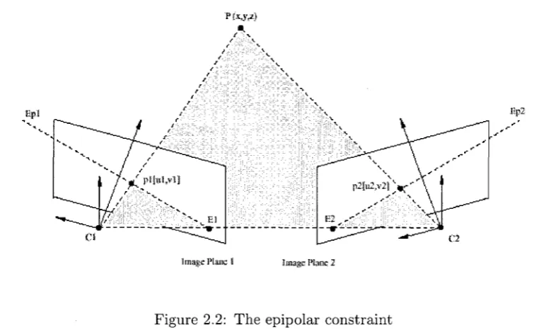
• Epipolar constraint: one of the most commonly used and useful stereo constraints in the literature that is also used in this work. It states that for each given point pi in the left image, the object point P projected onto point p lies somewhere on the ray that crosses points CI and pi. Projecting this ray onto the right image results in epipolar line defined by the corresponding point p2 and the epipole El. That is, the matching point of point pi lies on the corresponding epipolar line in the right image. Figure 2.2 shows a geometrical representation of this constraint.

*(*#*)

Image Hiu« I linage Plane 2

Figure 2.2: The epipolar constraint

• Smoothness constraint: this constraint (also referred to as continuity constraint) is widely used in stereo matching algorithms dictating that for each disparity estimated for a pixel, the neighboring disparity values do not abruptly change. Obviously, this assumption does not hold for disparities belonging to the object boundaries. There-fore, special considerations must be made to deal with such regions if this constraint is applied.

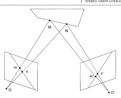
• Ordering constraint: The ordering constraint assumes that the order of points along the according epipolar line is preserved by the stereo projection, i.e. for a given point n on the right side of point m on the epipolar line, the matching point n' of n on

the other image must lie on the right side of the matching point m' of m as shown in Figure 2.3.

Figure 2.3: The ordering constraint

neighbor disparities. Second, this constraint does not always hold and is violated when we have thin foreground objects in the scene.

• Uniqueness constraint: This constraint states that for every point in the left image there is at most one matching point in the right image. It is based on the geometrical observation that it is impossible for an object point to project into more than one point (if non-occluded) in any given image. This constraint may be deployed to simplify the matching process or validate obtained results. One should note that this constraint is also violated when dealing with slanted surfaces as for such cases one point may be matched to many others.

• Visibility constraint: This constraint is originally designed in order to handle occlusion

and is derived from the definition of occlusion stating that a pixel in the left image will be visible in both images if there is at least one pixel in the right image matching it [37]. Visibility constraint is more general (and weaker) compared to both ordering and uniqueness constraints as it permits many to one matching, unlike the uniqueness constraint. Furthermore, the ordering constraint need not to be satisfied.

2.2 Stereo Matching Methodologies

As mentioned before stereo vision has been the subject of intense research for a long period of time (several decades). As a result, stereo vision literature is filled with a wide variety of methods developed with different level of efficiency and performance. Generally, most of these algorithms can be broadly categorized into local and global matching methods. Local methods typically calculate the disparity map using local image correlation over a certain area (window). Global methods on the other hand, model the disparity map constraints explicitly using energy functions and infer it through a global (usually iterative) optimization process. The following sections provide a brief review along with a comparison and analysis of both of the aforementioned matching algorithm categories.

2.2.1 Local M a t c h i n g

Local matching methods perform matching at a local level (hence the title local) and typi-cally involve the following steps:

1. Apply some dissimilarity measure to compute the pixel-wise matching cost

2. Aggregate matching cost over correlation window along the epipolar line within search window for all candidate disparity values

3. Determine the disparity based on WTA (Winner-Take-All) strategy, i.e. choose the disparity associated with the minimum cost at each pixel

4. Post-process results to remove outliers

Figure 2.4 depicts an example of performing local matching trying to find the corre-sponding point for a point p in the left image. As shown a local neighborhood of pixels surrounding point p is considered (the correlation window) in the left image. The same area (in terms of size and shape) is considered in the right image and is moved over for d different cases (d is the disparity range) along the epipolar line (presented as a dashed

line). The entire area in the right image covered by this process is called the search window. Each time the correlation window in the right image is moved, the new correlation value associated to that window is computed and stored. Finally, the displacement (disparity) producing the best (usually highest) correlation value is chosen.

i

Right

Figure 2.4: Pattern matching technique used in most local matching methods

2.2.2 Global Matching

Global matching methods formulate stereo matching problem in an energy optimization framework and are capable of yielding high quality results in the cost of being more com-plicated and therefore slower (as compared to local methods). Following is a summary of global methods features:

• Use stereo image pair as given evidence

• Often skip cost aggregation step

• Enforce the matching constraints through some potential functions incorporated into the energy function as shown in Equation (2.1):

- Data term measures how well estimated disparity agrees with the input image pair

- Smoothness term encodes smoothness assumptions regarding the disparity map

• Compute disparity map using a global optimization method (either ID or 2D) to find the disparity map corresponding to the minimum energy level

(2.1)

p

Left

D = argmirid E(d)

E(d) = EData{d) + \ESm,ooth{d)

The data term Er)ata(d) used in the energy function (also referred to as likelihood within

the Bayesian framework) is a measure of how well the disparity function d(x, y) agrees with the stereo image pair. It is computed based on the C(x,y,d(x,y)) function, which is the initial (or aggregated) matching cost function calculated in the previous steps. The data term is generally denned as follows [12]:

EData{d) = Y,x,yC(X'y>d(X>y))

The Esmooth(d) is the second term typically incorporated into the global energy

func-tion, which encodes the smoothness assumptions regarding the desired disparity map. Many global matching methods keep the smoothness function simple (e.g. by measuring only the differences between neighboring pixels disparities) in order to make the following optimiza-tion process computaoptimiza-tionally tractable. Equaoptimiza-tion (2.2) presents a generalized form of the smoothness function commonly used in the literature [12].

(2.2)

Esmooth(d) = Ex,B P(d(x, y) - d(x + 1, y)) + p(d(x, y) - d(x, y + 1))

The p is typically a monotonically increasing function of the disparity difference. If de-signed poorly, the smoothness term may smooth the disparity map everywhere and therefore lead to poor results at object boundaries. Global matching methods that rely on robust smoothness function and do not have such an issue are called Discontinuity — preserving. An example of such robust functions is illustrated in Equation (2.3), which relies on the pixel intensity differences to reduce the smoothness costs at high intensity gradients [12].

(2-3)

ESmooth{d) = E x ,y p(d(x> v) ~ d(x + J> v))-Pi(\!-*"0s. v) ~ J(x + 1, y)||) + p(d(x, y) - d(x, y +

The above formulation is based on the observation that object boundaries (depth discon-tinuity regions) usually coincide with the sudden changes in image gradients (edges). Thus to preserve depth discontinuities the smoothness term should not penalize such regions; i.e. pi is a monotonically decreasing function of intensity differences.

Examples of the smoothness functions widely used in the literature are truncated linear and quadratic model [12], the Potts model (also symmetric version) [42], and more recently the differential geometry consistency based method that is based on surface normal instead of the individual disparity values and can successfully recover both slanted and curved surfaces in the scene [43].

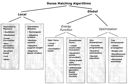
In majority of the global matching methods the main focus has been on improving the cost function optimization (i.e. minimization) step. In fact, there are numerous global stereo matching algorithms each based on a different energy optimization approach. These approaches can be further divided into ID and 2D optimization methods depending on the level at which optimization is performed. In ID methods such as dynamic programming [8], scanline optimization [44], and genetic algorithm [45] the optimization is performed for pixels within the image scanline at a time. In contrast, in 2D methods such as simulated annealing [47], belief propagation (BP) [1], graph cuts (GC) [2], and synchronous optimiza-tion [46] the entire image is considered at once. For example, in BP-based methods the disparity surface is modeled as a Markov random field (MRF). Then, assuming a Bayesian inference framework, the minimum energy level of the matching cost function corresponding to the Maximum A Posterior (MAP), i.e. the most probable disparity surface given input stereo image pair as evidence, is obtained deploying belief propagation approach iteratively. Figure 2.5 shows a summary of stereo matching categorization discussed here.

geomet-Local

Dense Matching Algorithms

Global Dissimilarity Measure: • Euclidean •Manhattan •Cross Correlation •Non-parametric transforms •Gradient based • LoG •Mean Correlation Window: • Rectangular • Adaptive window • Multiple window •Adaptive support weight • Segment-based window Energy Function Data Term: • Pixel -based •Correlation-based Smoothness ; Term: • Linear model (also truncated) •Quadratic model (truncated) •Potts model (also symmetric) • Differential geometry model (surface normal) Optimization One Dimensional: • Dynamic programming •Scanline optimization •Genetic algorithm Two Dimensional: • Belief propagation •Graph cuts •Simultaneous optimization •Simulated annealing

Figure 2.5: Summary of dense stereo matching methodologies

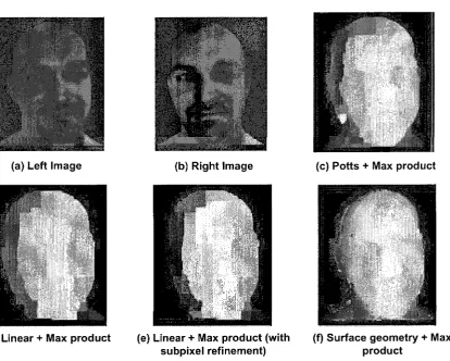
ric consistency as smoothness term, which helps eliminating the systematic error associated with modeling slanted and curved surfaces (common in the majority of matching algorithms assuming only fronto-parallel surfaces). This new method enforces geometric consistency for both depth and surface normal [43]. The experimental results presented in Figure 2.6, prove the efficiency and superior performance of this improved cost function in recovering depth information of human face as compared to two of the models commonly applied in the literature; i.e. truncated linear and Potts model. In all cases Bayesian belief propagation in max-product mode is used to estimate the MAP of the matching cost function.

2.2.3 Local vs. Global

dispar-(a) Left Image (b) Right Image (c) Potts + Max product

(d) Linear + Max product (e) Linear + Max product (with (f) Surface geometry + Max

subpixel refinement) product

Figure 2.6: Comparison of the surface geometry model to the truncated linear and Potts models [43]

Table 2.1: Brief comparison of local vs. global matching methods

Methodology Local Global

Emphasis Matching cost computation disparity computation Cost aggregation

Advantages Fast and efficient implementa- High quality results tion Easy to incorporate

con-straints

Drawbacks Window size and shape determi- Complicated

nation is difficult Slow Less accurate

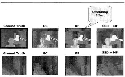
Global matching methods have the advantages of being capable of producing high qual-ity results, and ease of incorporating new constraints regarding the desired disparqual-ity map into the cost function. Figure 2.7 shows the disparity maps produced by applying two global matching algorithms (i.e. BP and GC) and a local matching method (sum of squared dif-ferences + mean filter) to tsukuba and venus image pair taken from Middlebury stereo webpage [48]. Results of dynamic programming approach are also included. One can see that due to considering only one scanline at a time, this method has difficulty maintaining consistency of results between image rows. A problem typically referred to as "streaking effect". Comparing the obtained results to the ground truth, it is clear that global match-ing methods are able to properly recover fine details of the scene whereas local matchmatch-ing methods have more difficulty dealing with object boundaries and textureless regions and therefore produce less reliable results.

Ground T r u t h GC

Ground T r u t h GC

DP

BP

S t r e a k i n g Effect

SSD + MF

SSD + MF

Figure 2.7: Qualitative comparison of local vs. global matching methods

discussed in chapter 3. Table 2.1 provides a brief comparison of local and global matching algorithms highlighting the main features for each group.

2.2.4 State of the Art

As mentioned in section 1.1, stereo vision research community has experienced significant contributions, mainly throughout the last couple of years, and many new high performance matching methods now exist in the literature. Most of these top-notch methods are global matching methods that deploy well-defined and robust cost (energy) functions along with an efficient optimization (inference) algorithm to compute the disparity map. Following is a summary of the main features/assumptions found in state of the art methodologies:

• Input image pair is assumed to be rectified

• Most of the methods have only considered static scenes

Cones

* *"H^

i i'

v*:

U-f

••-":•;

L£

m.

"••T- ~-i *

- ; • * • 1 .

r*i'.

i.

^^

:u

' S :

* " *

. _

t j

,

*»-^ - • : ] : . : i.

-"--:- • . ' A

"= : « :.:.'^ ' • - - . " ' : - • t\-'-f.

-••' - V " .- • J f?: -. •V; ! -1 L..u

Tsukuba

•*>i'v C> I . " V ' % i

jjt

Teddy

Venus

Figure 2.8: Test image pairs used in the Middlebury ranking of stereo matching methods

• Depth discontinuity areas are the most challenging regions resulting in highest error rates

• Most of top-performing methods rely on Bayesian belief propagation as inference method

• Recent methods attempt incorporating color segmentation data, enhanced similarity metrics, and cost functions to improve results

• Most of the them are computationally expensive and therefore relatively slow

Error Threshold

| E r r o i T h r e s h o l d .

Algorithm

AcfaMirwjBP n 31 DouiteleBPIISl Symap+occ 17] Seqm+visib [4] C-S£nrii«ob f1 SI RecjionXreeDP [18] EnhaiKedBP [241 AdaptWleicirrt[1 21 SeaTresDP 1221 lmprotreSubPix[25] SBBSlOfOt) J« RealtitneBP [21] = 1 i^l\ Avg. Rank

1

Sort by nonocc

V

ground truth

nonocc all disc

T

1-B I M l4 1-372 s7 3*

2 5 1 0 , 8 8 1 1.29 1 4.76 1 S.8 6 3 8 8 8 1 S 3 8 9 3.7 1 0 2

11.3

1 2 4

0,37:? 1 7 5 6 5 0 8 3

Venus

Sort by all

V

0.71 8 0 4 8 ? 0.88 11 ,1 00 M 0.77 j aM If azit 0.60 6 0.33 s 1.06 s 0 57 s 0.57 s 0 8 6 7 1.19 8 O60-5 1.47 10 1 . 5 7 f i 1.90 14

disc

1,44 t

2.00 0 2 1 8 4

Teddy

Sort by disc

W

ground truth

nonocc all

f

4.222 7.062 3.55 1 8.713 S 4 7 e 10,7 4 6.76 11 j 5.00 3 6.54 1 3 2 4 s \ 5 1 4 4 1 1 B *

r

1.932 7.42 ID 11.96 4.34s 8 S.11 12 1 3 3 10 6.139 7.88 11 13.3 n

2.445 -9.5816 1 5 2 1 5

7 . 1 0 ) . 11.317 9.00 16

7.12-) 12.40 6 0 2 s 1 2 . 2 / 8.72 15 1 3.2 •}

disc

1 1 8 2 9.70 '

i r o »

12.33 1 3 0 4 16.8? 18 512 18.6 14 18.4 11 16.6 Si Cones ground truth

nonocc all disc

2 . 4 8 1 7.922 ? . 3 2 i 2.90 3 9.24s 7.802 4 7913 10.71a (0.99 3.72? 8.625 10.2 = 2 77 2 8 35 4 8 20 3 6.31 1? 11.9 is 11.81^ S.PS t i 11.1 « 1 1 0 i o 3.97 s 9.79s 8.264 3 j 3 e 7 . 8 6 1 3.83 s 2.96 4 8.22 -j 8.55; 1 S 3 ^ . 3,B6« 9,757 8 9 0 ? 17.20 4.61 11 11.613 12.4 18

Figure 2.9: Latest ranking of state of the art stereo matching algorithms [48]

The percentages of mismatches (erroneous matches) B for each category is computed by counting the number of pixels for which the estimated disparity values differ from the correct one (determined by the ground truth) by more than a threshold value 5a [12] as shown below:

B = 7i^2(x,y)(\dc(x,y) - dT{x,y)\ > 5d)

Real-time Stereo Vision

3.1 Fast Stereo Matching

Numerous stereo matching algorithms with real-time or near real-time performance exist in the stereo research community. These algorithms can be generally classified into two groups: area-based methods and feature-based methods. Feature-based methods operate by extracting viewpoint invariant features (e.g. edge, corner, and line segment) from the image and trying to match them. They have very fast and efficient implementation, however, can only yield a sparse disparity map. Area-based methods calculate disparity map using local image correlation over a certain area (window). They are usually preferred as they can find a dense disparity map in contrast to the feature-based methods.

Figure 3.1: SRI small vision module [56]

realize high quality yet real-time stereo vision systems and algorithms [50, 51, 52]. As mentioned in section 2.2.3, DP has the advantage of performing the optimization in a one-dimensional manner (along the scanline) in contrast to the more complex two-one-dimensional optimization of BP and GC based methods. Nevertheless, as previously discussed it has drawbacks such as suffering from erroneous horizontal strokes (streaking effect) as well as being unable to deal with vertical displacement between input images [50]. On the other hand, local matching methods especially correlation-based matching techniques have already proven to be a feasible solution for real-time stereo in various software [53] and hardware applications [54,55].

3.1.1 Correlation-based Matching

As mentioned in the previous section, correlation-based stereo has a long history of being used as real-time stereo matching solution in numerous applications. It consists of four main steps;

1. Use some dissimilarity measure to compute pixel-wise matching cost (Manhattan and Euclidean distances are the most commonly used measures deployed in this step).

search window.

3. Determine initial disparity map by finding the best disparity candidate through Winner-Take-All (WTA) strategy.

4. Post-process obtained results to remove potential outliers or produce sub-pixel dis-parity estimates.

While some algorithms in this area try to improve the accuracy of the correlation-based stereo through incorporating constraints such as ordering, uniqueness, and visibility into the matching process [37, 57], more recent methods take a more systematic approach and develop more advanced pixel dissimilarity metrics and/or cost aggregation methods to enhance the overall performance of the matching algorithm in problematic areas such as poorly textured regions and disparity discontinuity regions [39, 24, 58, 23].

Performance of the correlation-based matching algorithms is highly dependent on the cost aggregation approach deployed. Indeed several new cost aggregation methods have been proposed in the literature that produce higher quality results than many global matching methods [?, 60, 39]. Although, some of these methods can not achieve real-time perfor-mance. A recent study provides a comparison of several aggregation methods in terms of both computational cost and quality of disparity maps produced [59]. The conclusive remakes presented, serve as useful guidelines for developing novel real-time stereo vision systems. For example, it is shown that sampling insensitive matching method [36] and shiftable windows, commonly used in offline stereo matching algorithms, are of no benefit for real-time applications. It is due to the fact that for the sake of the processing speed, majority of real-time stereo algorithms represent matching costs as single bytes. As a result, small cost differences can not be distinguished due to the limited available precision.

Figure 3.2: Miniature Stereo Vision Machine based on FPGA (MSVM III) [3]

1

Figure 3.3: The Acadia-I PCI vision accelerator board [71]

The proposed algorithm objective is to develop a stereo matching method that produces ac-curate results (especially at object boundaries), is invariant to illumination changes (due to application of the mutual information), and can be implemented efficiently. In their paper, authors first introduce a hierarchical scheme for computation of mutual information based matching, which makes it virtually as fast as intensity based matching. Then, propose a semi-global matching method, which is basically an approximation of global cost calculation with linear complexity with respect to the number of pixels and disparities.

3.2 Previous Work

up to 60 fps [3] (see Figures 3.2 and 3.1). Some researchers have also attempted utilizing the VLSI technology for developing application specific integrated circuit (ASIC) based vision systems. Acadia vision processor is an example of such systems illustrated in Figure 3.3. However, due to their high cost, lack of flexibility, and rather time-consuming and compli-cated design process, such systems are rarely implemented. Several PC-based stereo vision systems have also been recently reported that achieve their efficiency through incremental calculation schemes aimed to avoid redundant calculations and parallelizing the computa-tionally expensive portion of the algorithm with Single Instruction Multiple Data (SIMD) parallel instructions, available nowadays in almost any state-of-the-art general purpose mi-croprocessors [5] or utilizing the vector processing capability and parallelism in commodity graphics hardware to speed up the matching process [8].

Miniaturized Embedded Stereo Vision

System (MESVS)

4.1 System Overview

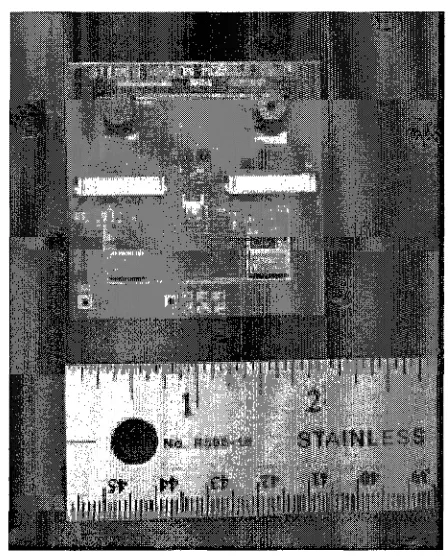
This chapter describes the design and implementation of a new miniaturized and fully integrated embedded stereo vision system (MESVS) developed for this thesis. The MESVS vision system is compact, power-efficient and of low-cost and is based on the state of the art dual core embedded media processor as computational platform. The main aim of this work has been to develop a small, efficient, real-time, and intelligent stereo-vision sensor that can be applied in a wide variety of imaging applications in real-world environments. The MESVS shown in Figure 4.1, fits within a tiny package of only 5x5cm, is capable of producing accurate and quality disparity maps at 20fps while operating at 600MHz per core. Furthermore, it is quite power-efficient and consumes very low power (i.e. [email protected]).

The system firmware consists of five main steps as follows:

1. Image sub-sampling

Figure 4.1: Miniaturized Embeddded Stereo Vision System developed for this work

3. Pre-processing step based on local non-parametric transforms

4. Correlation-based matching with three levels of recursion followed by cross checking to detect and remove half-occluded regions of the scene

5. Novel postprocessing algorithm to improve obtained results around object boundaries and reduce number of mismatches caused by low-texture areas

The high level of performance, quality and accuracy of MESVS firmware was achieved through efficient implementation of the algorithms, improved memory and data manage-ment, in-place processing scheme, careful code optimization, and deploying pipe-lined pro-gramming model, that leverages the advantages of dual-core architecture of the embedded vision processor used.

and limitations of embedded settings and also design aims of the system such as real-time performance and high accuracy are discussed.

4.2 Hardware Description

4.2.1 Horopter vs. range accuracy analysis

As mentioned before the major focus of this work has been on keeping the overall dimensions, power consumption and cost of the system as small as possible, while improving the accuracy and performance. One of the impacts of miniaturizing the dimensions of the system is on the baseline, i.e. the distance between cameras centers of projection. Regarding the system dimension of only 5x5 cm and based on results of the following analysis, the baseline of about 28mm was chosen for the system. In fact, the small focal length of the compact camera modules along with the small baseline, necessitates analyzing the resulting effect on the range of measurable objects in the scene (Horopter) and also the corresponding accuracy (range uncertainty) to evaluate the feasibility of such a configuration. Technically, the horopter must be large enough to encompass the range of objects in the application. Furthermore, the corresponding range accuracy associated with the obtained disparities within the specified horopter must be acceptable.

As shown in Equation 4.1 the range uncertainty Ar is proportional to the range r, baseline 6, focal length / , pixel size x, and the change in disparity AN. Regarding a baseline of 28mm, focal length of 28mm, and pixel size of 17um, setting system horopter to 5-35 pixels with disparity range of 30, yields a measurable range of about 15-100 cm (see Figure 4.2).

(4.1)

Ar = (^)xAN

120 11D 100 90 SO

I 7°

I 5» 40 30 20 10 \ \ \ \ ,

Range vs. Disparity

v-^ . -'

15 20 25 Disparity (pixels)

Figure 4.2: Analysis of range versus corresponding disparity

25

20

f

u | 1 5

c <y

= 10

5

n

Range uncertainty vs. Range

/ / -y /' y s ' ,-•' ^ ^'"^"" ,"-"''''' „..^--"""""

10 20 3D 40 50 60 70 BO 90 100 110 Range(cm)

Figure 4.3: Analysis of range uncertainty versus corresponding disparity

(4.2)

Nx

4.2.2 Choice of computational platform

Another important item that was carefully chosen is the hardware technology used as com-putational platform as it heavily influences the cost, performance, and the power consump-tion characteristics of the final system. Following is a list of the criteria taken into account for choosing the appropriate computational platform for this work:

• Performance characteristics (i.e. processing speed, memory architecture and features, data buses, power requirement, benchmark results, etc.)

• Development considerations (i.e. single vs. multi-core architecture, number and vari-ety of I/O ports and peripherals supported, instruction set features, developer famil-iarity and learning curve, compatibility, customer support, etc.)

• Cost of integration

• Availability and future roadmap

• Packaging considerations

extensive tuning. Their roadmap is also unclear and the benefits of low cost can only be realized when mass produced. FPGAs may seem like a promising alternative as they can be reconfigured dynamically, offer architectural flexibility, high throughput and performance; however, they have drawbacks such as requiring design skills beyond that found in many vision labs today [61], they also consume more power, cost higher [56] and have larger foot-print when compared to state-of-the-art embedded microprocessor solutions. Therefore, although FPGAs offer higher computational power, our embedded vision system is based on an embedded processor with integrated DSP functionality as the processing unit mainly due to its lower power consumption and compact size, which are of outmost importance regarding the design constraints of the system mentioned before.

4.2.3 Hardware implementation

of programming and performance versus cost and energy efficiency.

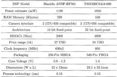
There are three main vendors of high performance fixed-point DSP processors: Ana-log Devices, Texas Instruments, and Freescale. AnaAna-log Devices ADSP-BF5xx (Blackfin), Freescale's MSC81xx and MSC71xx, and Texas Instruments TMS320C64x family of proces-sors are the three main competitors in the area of high performance fixed-point DSPs [62]. Although Freescale's MSC81xx and MSC71xx and Texas Instrument's TMS320C64x family of processors provide high performance levels (clock speed of up to 1GHz), they are not originally designed for multimedia applications and therefore do not support video cap-ture and processing facilities found in Blackfin processors. Additionally, they are not as power-efficient as Blackfin processors and cost more on average.

i.MX processors from Freescale and DaVinci processors from Texas Instruments are com-parable to Blackfin processors in the sense that both are designed for embedded multimedia applications and comprise in-built camera interface and video processing and enhancement sub-systems. The processors that support a digital camera interface have an advantage in terms of performance because the core processor does not have to care about low-level video synchronization and transfers. These interfaces all have DMA (Direct Memory Access) ca-pability, which is the only efficient way of handling the huge amount of video data with no intervention of the core processor. This way, core processor can analyze a frame in the main memory while the DMA can grab the next frame and move it to the main memory [63]. i.MX processors only support one camera interface and therefore may not be used to imple-ment stereo vision system, which requires at least two interfaces. DaVinci processors supply more processing power than Blackfin family (up to 7200 MMACs@900MHz), yet they cost more and also have higher power consumption and larger dimensions. As a result, Blackfin family of processors is the best choice regarding the aforementioned design requirements of MESVS.

Table 4.1: Comparison of the embedded processors DSP Model

Power estimate (mW) RAM Memory (Kbytes)

Camera interface Architecture MMACs (Max) Price range (Ik) Clock frequency (MHz)

Packaging Core Voltage (V) Dimensions (W x L) Process technology (um)

Blackfin ADSP-BF561

1100 328

2 (ITU-656 compatible) 16 bit fixed-point

2400 27 USD

600x2 256-Pin MBGA

0.8- 1.2 12 x 12mm

0.13

TMS320C6418-600

1850 548

2 (ITU-656 compatible) 32 bit fixed-point

4800 55 USD

600 548-Pin PBGA

1.4 23.1 x 23.1mm

0.13

as much, occupies almost four times more space and requires more power. The processors have some features in common such as supporting two camera interface ports compatible with ITU-R656 video signaling standard, being based on 0.13um CMOS technology, and operating at up to 600MHz. Considering the major requirements of our design, i.e. power efficiency, compactness and low cost, ADSP-BF561 has been chosen as the processing unit of our system.

CAMERA PAIR

C A M 1

(left)

a

VGA (640K480)

C A M 1 p - 0V7660

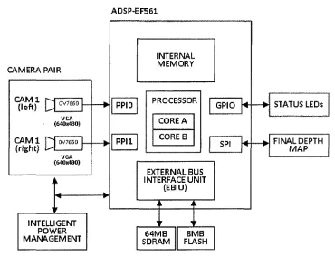
(right) VGA (640x480) <#-INTELLIGENT POWER MANAGEMENT ADSP-BF561 PPIO PPI1 INTERNAL MEMORY PROCESSOR CORE A COREB EXTERNAL BUS INTERFACE UNIT (EBIU) 64MB SDRAM 8MB FLASH GPIO SPI

-W STATUS LEDs

FINAL DEPTH MAP

Figure 4.4: High level block diagram of MESVS

bottlenecks in video data movements within the system and keep the core processors away from performing slow memory accesses. The MESVS also includes 64 MB of SDRAM, 8 MB of addressable flash memory, and dynamic core voltage regulator that allows adjusting core voltage through software. Furthermore, system board is hosting two camera modules and their corresponding oscillators, and voltage regulation circuitry to allow standalone operation of the system. A JTAG interface is also incorporated used for debugging and downloading system firmware. Finally, the SPI port is used to enable connection of the embedded stereo vision system to the other units (modules) within an embedded setting.

Left Image Right Image

Figure 4.5: Sample stereo snapshots captured by the CMOS camera modules

DSP of the camera provides some basic image processing functionality such as auto expo-sure and white balance control, color and gamma correction, and color space conversion, e.g. from RGB to YUV color space. ITU656 is a digital video protocol that requires video timing signals such as horizontal and vertical synchronization signals to be embedded as reference codes within video data stream. This in turn results in simpler and more robust video capture process. The camera module was set to supply the graphic data in the YUV 4:2:2 format. To reduce the image size and the computational burden, only the luminance channel Y data is used and the captured images are stored as grayscale. Figure 4.5 shows sample binocular snapshots taken by the system.

4.2.4 Memory architecture

high-ADSP-BF561

m

m

L I MEMORY (32KB} ;

INSTRUCTION

SKAM/CACHE M M U

II

: :Jfe. CORE 2

14 MEMORY

~*\ DATA SRAM/

CACHE

L I MEMORY (32KB) INSTRUCTION

SRAM/CACHE M M O

OATA SRAM/ V CACHE• i

m

CORE SYSTEM/BUS INTERFACE P I M O M A c o y o t e s

324 External Access BusfEAB) BOOT ROM: CiFf-CHiP 4.32: DMA Controller 1 DMA : External BusfOEB). DMA: Access Bus (DAB); 4 3 2

m

t T t t t T t t t t t T

NfSMAPERIPHERALS ; EXTERNAL PORT

FLASH/SDRAM CONTROL 64MB SDRAM; >6DpMHz CdreClbek : (CCLK) domain Single cycle t o access

>3Q0MHz

System Clock :

(SCLK) domain Several cycles: t o access

<e=133MHz SeveralSystem cycles t b access

Figure 4.6: Overview of memory architecture of the MESVS

64MB of SDRAM and 8MB of flash memory. The systems firmware is burnt onto and kept on the flash memory through JTAG interface. The L3 memory is quite large. However, its access time is measured in System Clock Cycles (SCLK), which is usually much larger than the Core Clock Cycles (CCLK). Therefore, to assure optimum system performance, slow memory accesses to the external memory are mostly performed using DMA facility and majority of memory accesses of the processing cores is limited within the fast on-chip memory (LI nd L2) of the system as explained in section 4.3.3.

Blackfin architecture supports several DMA channels that facilitate data movement between the peripherals and also within memory unit, without causing overhead to the processing cores. The DMA features are extensively deployed in order to improve system performance and reduce the run-time of the stereo matching, and rectification algorithms as discussed in section 4.3.3.

4.2.5 Power consumption

In most of the embedded systems especially mobile platforms that rely on batteries as the sole source of energy, power management requires special consideration. Because stereo matching algorithms are computationally expensive, the system has to operate at maxi-mum capacity (system clock) in order to achieve a real-time processing rate. In addition, the matching algorithm must be carefully selected and tuned, to take advantage of the dynamic power management. Blackfin processors have the ability to vary the voltage and frequency dynamically, which facilitates reduction of power consumption. Dynamic power consumption is directly proportional to the square of the operating voltage VDD and linearly proportional to the operating frequency / , as shown in the Equation 4.3 [18, 21] below (K is the system constant):

(4.3)

- ' d y n a m i c = -"• ' £)D ' J

the lowest voltage allowed. Because lowering frequency also means that it takes more time for the firmware to execute. MESVS incorporates power saving features such as intelligent voltage regulation, dynamic management of frequency, flexible power management modes (sleep, hibernate, full-on and active), and isolated power domains for components. Having multiple power domains, one for the internal logic circuitry of the processor and the other for I/O, improves flexibility and power savings of the system. External components such as L3 memory chip were carefully selected, taking their power consumption into account. In addition, the IDE used to develop system firmware, i.e. Analog Devices's VisuaiDSP+-1-suite features a Statistical Profiler tool that can quantify exactly how much time is spent in any given segment of the firmware. Using this tool, the major segments of system firmware were carefully tuned to maintain a balance betwwen power demands and performance. Regarding all this, the average active power dissipation of MESVS is estimated (through adding the active power dissipated in individual power domains) to be about 2.3W (i.e.

[email protected]).

4.3 System Firmware

This section provides a detailed explanation of the development process taken to implement the firmware for MESVS. As briefly discussed in section 4.1, MESVS relies on a multi-step recursive correlation-based stereo matching algorithm to achieve high performance and quality results. In the next sections first the offline stereo calibration procedure is explained followed by an in-depth discussion of stereo matching engine (elaborating on each of the steps) in section 4.3.2. Finally, in section 4.3.3 the measures taken to enhance system functionality in order to attain real-time performance are presented .

4.3.1 Stereo calibration

wcs

'{%,y,x)

X /

Optical e&mr /

ze

/ Optical wm

Image Plane

Figure 4.7: Pinhole camera model

camera model and therefore is capable of calibrating a wide range of camera systems. T h e

camera model is very similar to t h a t used by [65]. It is based on t h e pinhole camera model

(see Figure 4.7) and considers b o t h radial and tangential distortions using five coefficients

(distortion model is also known as " P l u m b Bob" [66]). Furthermore, it naturally supports

square pixels and through estimation of skew factor allows the pixels to be even

non-rectangular. In addition to calculating estimates for the intrinsic camera parameters such

as focal length, projection center, pixel size, distortion p a r a m e t e r s and extrinsic stereo

parameters (i.e. rotation and transformation), the toolbox also r e t u r n s estimates of the

corners of the calibration pattern and software is able to extract the rest of the corners automatically, which in turn speeds up the calibration process. Figure 4.8 shows several snapshots of the calibration pattern used to calibrate the right camera module.

Through experiments, the stereo calibration process was found to be a difficult and rather time-consuming stage and very influential on the quality of the final disparity map obtained. In order to maximize the accuracy, we captured our calibration shots in the maximum resolution provided by our camera modules (i.e. VGA), which allowed to locate the four extreme grid corners in the most precise way possible. Moreover, the 3D positioning of the planar calibration pattern through the calibration shots must include a wide range of varieties along three axes (X, Y, and Z) and three orientations (pitch, yaw, and roll) to allow for external stereo parameters to be estimated with reasonable accuracy. Finally, it was proven experimentally that the radial distortion of the cameras must be compensated. Although, considering the tangential distortion in the model would slightly improve the results, it would considerably increase the computational complexity of the un-distortion algorithm. As a result, in the current implementation only radial distortion of the cameras is corrected in order to maintain a balance between performance and quality. One of the future avenues of research of this work would be to develop and implement an online self-calibration algorithm, which is necessary for the system to produce consistent and reliable results over the time.

4.3.2 Stereo matching engine

elab-Figure 4.8: Sample snapshots of the calibration pattern used to calibrate the right camera module

oration on each of these five steps.

Image sub-sampling

One of the main challenges of programming for a vision application in an embedded setting is the very limited amount of fast on-chip memory available compared to the size of the image and video data. Although external memory may also be deployed to store and retrieve image data, it typically operates at much lower speed compared to the processing core and the high access latencies associated to it would make system performance to suffer. That is, processing cycles would be wasted waiting for the new data to be supplied by the slow external memory.

Left Image VGA (640x480) OV7660 CAMERA 0 Offline Calibration i OV7660 CAMERA 1 Right Image VGA (640x480) SUB-SAMPLING Sub-Sampled Image QQVGA (160x120) RECTIFICATION PRE-PROCESSING CORRELATION BASED MATCHING POST-PROCESSING

FINAL DISPARITY MAP

Back Projection, Distor-tion Removal, Bi-Linear Interpolation

Rank Transform

ft

rhree-Level Recursion L/R Consistency Check

Removal of errors intro duced by depth discon-tinuities and low-texture regions

Figure 4.9: A step-by-step diagram of the stereo matching engine of MESVS

of the Blackfin processor by skipping every three rows and columns of the input image as shown in Figure 4.10.

Stereo rectification

Figure 4.10: Image subsampling from VGA to QQVGA using 2D DMA facility

for each of the pixels in the image the back projected coordinate in the rectified image is computed through a matrix multiplication using homogeneous coordinate system and then is converted back to the regular (Cartesian) coordinate system. The elements of the back projection matrix are based on the parameters estimated in the calibration step and

are real numbers (For more detailed explanation please refer to [67]). Therefore, this matrix should be represented using floating-point data meaning that implementing back projection step requires floating-point arithmetic.

(4.4)

1. for i — 1 to image height 2. for j — 1 to image width

2.1 rays = back projection matrix • [j i 1]

2.2 back projected coordinate = [rays(l, 1) / rays(3,1) rays(2,1) / rays(3,1)] 3. end