NUCLEAR RESONANCES
by
UNDRAA AGVAANLUVSAN
A dissertation submitted to the Graduate Faculty of North Carolina State University
in partial fulfillment of the requirements for the Degree of
Doctor of Philosophy
Department of Physics
Raleigh 2002
APPROVED BY:
Christopher R. Gould
John H. Kelley D. Ronald Tilley
Gary E. Mitchell, John F. Shriner, Jr.,
Undraa Agvaanluvsan
Personal:
Born 24 March 1973, Ulaanbaatar, Mongolia Married to Dugersuren Dashdorj, son Baljinnyam
Education:
B.S. in Physics, National University of Mongolia, 1994 M.S. in Physics, National University of Mongolia, 1995
Diploma in High Energy Physics, International Centre for Theoretical Physics, Trieste, Italy, 1997
Academic Positions:
Lecturer, National University of Mongolia, 1997-1998
Teaching Assistant, North Carolina State University, 1998-2000 Research Assistant, North Carolina State University, 2000-2002
I have been fortunate to be Dr. Gary E. Mitchell’s student. I am grateful to his teachings and involvement in my graduate study. I have learned much from him; this will be remembered and valued throughout my life. I am also thankful to my co-advisor Dr. John F. Shriner, Jr. for his insights and help while preparing my dissertation.
I thank Dr. Mauricio Pato for his partnership in my research. I appreciate Dr. Chris-ten M. Frankle for providing valuable data for my analysis. Special thanks are due to Dr. Christopher R. Gould for his inspiration and belief in my abilities. I thank Dr. John H. Kelley and Dr. D. Ronald Tilley for kindly agreeing to serve on my thesis committee. Thanks to my fellow graduate students Bill Beal, Daniel McDevitt, Lance McLean, and Stephen Lokitz for a friendly work environment and good humor, and Emel Tavukcu for her friendship.
I am eternally thankful to my father Agvaanluvsan and mother Battogtokh for their great love that I feel even this far away. I also thank them for their high expectations. I thank my dear son Baljinnyam for his patience with my busy schedule during this graduate study. His sweet support has always been truly touching. I thank my brothers Hudree, Idree, and my sister Indraa for their love, trust, and respect. Last, but not least I wish to thank my husband Dugersuren Dashdorj for his love and support. I specially thank him for his ability to help me stay focused on what is important in life.
List of Tables vi
List of Figures viii
Chapter 1 Introduction 1
Chapter 2 Level Densities 5
2.1 Historical background . . . 5
2.2 Random matrix theory . . . 8
Chapter 3 Width Analysis of Imperfect Sequences 12 3.1 The standard iterative method . . . 13
3.2 An example of the iterative method . . . 16
3.3 Advantages and disadvantages of the standard iterative method . . . 17
3.4 The maximum likelihood method . . . 18
Chapter 4 Spacing Analysis of Imperfect Sequences 20 4.1 Derivation of the PDF . . . 21
4.2 Theoretical GOE sequences . . . 26
4.3 The k-th nearest neighbor spacing distributions . . . 30
4.4 Spacing distributions for imperfect GOE sequences . . . 34
5.1 Proton resonances . . . 40
5.2 Neutron resonances . . . 43
Chapter 6 Analysis of Resonance Data 45 6.1 Introduction . . . 45
6.2 Missing levels . . . 45
6.2.1 Width analysis . . . 45
6.2.2 Spacing analysis . . . 49
6.3 Spin misassignments . . . 59
Chapter 7 Data and Analysis 63 7.1 Proton resonances in p +44Ca . . . 63
7.2 Proton resonances in p +48Ti . . . 67
7.3 Proton resonances in p +56Fe . . . 71
7.4 Neutron resonances in n +64Zn and n +238U . . . 71
Chapter 8 Results 83 8.1 Level densities . . . 83
8.2 Angular momentum dependence . . . 83
8.3 Parity dependence . . . 89
Chapter 9 Summary and Conclusions 91
Bibliography 94
Appendix A Proton Resonance Energies and Reduced Widths 100
Appendix B Spacing Anomalies 116
Appendix C Unfolded Sequences 132
3.1 Dependence of missing fraction and strength on the cutoff. . . 14
3.2 Missing fraction for p +48Ti 12+ resonances. . . 17
4.1 Calculated values for p(1;x) and p(2;x). . . 32
6.1 Large spacing anomalies in p +48Ti 12+ resonances. . . 54
6.2 Percentage of levels with spacings≥x. . . 54
6.3 Percentage of levels with spacings≥1/x. . . 61
6.4 Small spacing anomalies in p +48Ti 12+ resonances. . . 62
7.1 Observed fractionf for p +44Ca resonances via width analysis. . . . 64
7.2 Observed fractionf for p +44Ca resonances via spacing analysis. . . . 64
7.3 Large spacing anomalies in p +44Ca resonances. . . . 66
7.4 Small spacing anomalies in p +44Ca resonances. . . . 68
7.5 Level densities and proton strength functions for the p +44Ca reaction. . . 69
7.6 Observed fractionf for p +48Ti resonances via width analysis. . . 69
7.7 Observed fractionf for p +48Ti resonances via spacing analysis. . . 69
7.8 Large spacing anomalies in p +48Ti resonances. . . 70
7.9 Small spacing anomalies in p +48Ti resonances. . . 72
7.10 Level densities and proton strength functions for the p +48Ti reaction. . . . 73
7.13 Large spacing anomalies in p + Fe resonances. . . 74
7.14 Small spacing anomalies in p +56Fe resonances. . . 74
7.15 Level densities and proton strength functions for the p +56Fe reaction. . . . 75
8.1 Summary of level densities for p +44Ca, p +48Ti, and p +56Fe. . . 84
8.2 Proton strength functions for p +44Ca, p +48Ti, and p +56Fe. . . 85
8.3 Parity asymmetry in the proton resonance level densities. . . 89
A.1 p +44Ca 1 2 + resonances. . . 101
A.2 p +44Ca 1 2 − resonances. . . . 102
A.3 p +44Ca 3 2 − resonances. . . . 103
A.4 p +44Ca 3 2 + resonances. . . 104
A.5 p +44Ca 5 2 + resonances. . . 105
A.6 p +48Ti 12+ resonances. . . 106
A.7 p +48Ti 12− resonances. . . 107
A.8 p +48Ti 32− resonances. . . 108
A.9 p +48Ti 32+ resonances. . . 110
A.10 p +48Ti 52+ resonances. . . 111
A.11 p +56Fe 12+ resonances. . . 112
A.12 p +56Fe 12− resonances. . . 113
A.13 p +56Fe 32− resonances. . . 113
A.14 p +56Fe 3 2 + resonances. . . 114
A.15 p +56Fe 5 2 + resonances. . . 115
3.1 Cutoff dependence of the missing fraction and strength . . . 15
4.1 Examples of theN −1 expression. . . 25
4.2 Nearest neighbor spacing distribution. . . 28
4.3 Effect of GOE size on NNSD. . . 29
4.4 k= 1 andk= 2 nearest neighbor spacing distributions. . . 31
4.5 Interpolation vs. Gaussian for p(1;x) and p(2;x). . . 33
4.6 Truncation of the summation over k. . . 35
4.7 NNSD for imperfect GOE sequences. . . 36
4.8 Maximum likelihood function for spacings. . . 37
4.9 Dependence of the likelihood function on statistics. . . 38
5.1 Jπ resonance shapes for various detector angles. . . . 42
6.1 Maximum likelihood function for p +48Ti 12+ resonance widths. . . 47
6.2 Reduced width distribution for p +48Ti 12+ resonances. . . 48
6.3 Non-statistical effect on the reduced width distribution. . . 50
6.4 Width distribution with analogs removed. . . 51
6.5 Fit to the integrated level density N(E). . . 53
6.6 Spacing anomalies in p +48Ti 12+ resonances. . . 55
6.9 NNSD and cumulative spacings for p +48Ti
2 resonances. . . 60
7.1 Sum of reduced widths and number plot for 12+ resonances in n +64Zn. . . . 76
7.2 Reduced width distribution in n +64Zn 12+ resonances. . . 77
7.3 NNSD for 12+ resonances in n +64Zn. . . 78
7.4 Sum of reduced widths and number plot for 12+ resonances in n +238U. . . . 79
7.5 Reduced width distribution in n +238U 12+ resonances. . . 80
7.6 NNSD for 12+ resonances in n +238U. . . 81
8.1 J dependence of level densities in p +44Ca. . . 86
8.2 J dependence of level densities in p +48Ti. . . 87
8.3 J dependence of level densities in p +56Fe. . . . . 88
8.4 Parity asymmetry in the proton resonance level densities . . . 90
B.1 Spacing anomalies in p +44Ca 1 2 + resonances. . . 117
B.2 Spacing anomalies in p +44Ca 1 2 − resonances. . . . 118
B.3 Spacing anomalies in p +44Ca 32− resonances. . . 119
B.4 Spacing anomalies in p +44Ca 32+ resonances. . . 120
B.5 Spacing anomalies in p +44Ca 52+ resonances. . . 121
B.6 Spacing anomalies in p +48Ti 12+ resonances. . . 122
B.7 Spacing anomalies in p +48Ti 12− resonances. . . 123
B.8 Spacing anomalies in p +48Ti 32− resonances. . . 124
B.9 Spacing anomalies in p +48Ti 32+ resonances. . . 125
B.10 Spacing anomalies in p +48Ti 52+ resonances. . . 126
B.11 Spacing anomalies in p +56Fe 1 2 + resonances. . . 127
B.12 Spacing anomalies in p +56Fe 1 2 − resonances. . . . 128
B.13 Spacing anomalies in p +56Fe 3 2 − resonances. . . . 129
B.14 Spacing anomalies in p +56Fe 3 2 + resonances. . . 130
C.1 Fits to the integrated level densityN(E) (part 1). . . 133
C.2 Fits to the integrated level densityN(E) (part 2). . . 134
C.3 Fits to the integrated level densityN(E) (part 3). . . 135
C.4 Fits to the integrated level densityN(E) (part 4). . . 136
C.5 Fits to the integrated level densityN(E) (part 5). . . 137
C.6 Fits to the integrated level densityN(E) (part 6). . . 138
Introduction
The average properties of energy levels are important for many reasons, including the study of nuclear reactions, of nucleosynthesis, and of other aspects of astrophysics. Nuclear reactions may be classified into two major classes, fast and slow. In the first case a typical reaction time is so short that the interaction takes place with only one or a few nucleons inside the nucleus. In such cases the coherence and interference effects between incoming and outgoing nucleons are strong.
Another extreme is provided by the slow reactions where the typical reaction times are several orders of magnitude longer. The incident nucleon is trapped and all of its energy and momentum are quickly distributed among the various constituents of the target nucleus. The target nucleus and the incident nucleon form a “compound nucleus.” The compound nucleus lives long enough to forget the details of formation, and the subsequent decay is independent of the manner of its formation. The compound nucleus is formed above the separation energy; at this rather high excitation energy the level density is usually large. Due to the large number of neighboring energy levels of the compound nucleus (and the complexity of their wave functions), there is a focus on average properties, such as the average strength and spacing. It is natural that such phenomena, which result from complicated many body interactions, will give rise to statistical theories.
proposed to explain nuclear behavior. Bethe [Bet37] derived a useful form for the energy and spin dependence of the level density based on a Fermi gas model and simple counting arguments. The independent particle model, in which nucleons are assumed to move freely in an average potential, has been successful in predicting the bound state structure of various nuclei.
For a simple quantum mechanical system, one attempts to specify all interactions through a Hamiltonian H, and solves the Schrodinger equation Hψλ = Eλψλ. When the
system is sufficiently small, one can solve the equation and determine the nuclear levels. However, as the excitation energy is increased, the number of possible configurations be-comes very large, and the exact solution of the Schrodinger equation is impossible. It is under these circumstances, where the structure is very complicated (high level density), that a statistical analysis is suitable. Of course, there is nothing statistical about the nuclear interaction. One justification for the statistical approach is empirical – it works. A more general justification in terms of a quantum chaos description of the strongly interacting many body system remains a topic of active theoretical interest.
New theories may provide an accurate description of existing data as well as an improved physical understanding of the relevant level density parameters. A recent calcula-tional method based on Shell Model Monte Carlo (SMMC) [Lan93, Nak98, Alh99] techniques makes predictions for level densities, and the results appear promising. Showing that these calculations can correctly describe existing data would provide increased confidence for level density predictions far from stability.
from resonance data.
The standard method for the missing level correction involves resonance widths. In this approach one assumes that the resonance widths obey a Porter-Thomas distribution and that all levels below some cut-off are not observed. This approach works fairly well but it has several limitations. In order to determine the most reliable correction for missing levels, an additional method is needed. The Porter-Thomas distribution follows from Random Matrix Theory (RMT) [Guh98]. Another prediction of RMT is that the nearest neighbor spacings for a set of states with the same symmetry properties obey the Wigner distribution. Since in RMT the widths and spacings are not correlated, analysis of the spacing distribution can provide an independent determination of the missing fraction of levels.
Since the spacings are missed at random, the effect of missing levels on the spac-ing distribution is complicated. Because of this complexity, corrections usspac-ing the detailed spacing analysis approach have essentially never been performed. A new method that we developed provides a general expression for the spacing distribution for sequences with missing levels. We have also developed a practical analysis method using this distribution. This work consists of 9 chapters and 3 appendices. A brief historical background for level densities and a theoretical introduction to RMT are discussed in the following chapter. The standard width analysis is summarized, and an improved width analysis is described in chapter 3. The next chapter includes a derivation of the spacing distribution for imperfect sequences, as well as the results of testing this distribution with numerical simulations.
Level Densities
2.1
Historical background
Nuclear level densities play an important role in estimating nuclear reaction rates in general, and for nucleosynthesis and reactions involving unstable nuclei in particular. In 1936 Bethe published his landmark work [Bet36] presenting the well-known Bethe formula for nuclear level densities. This Constant Temperature Formula (CTF) was based on a Fermi gas model of the nucleus:
assumption (ii) is not completely valid for the nucleus [Mar41].
In order to account for these effects, several phenomenological modifications of this simple formula have been proposed and used for comparison with experimental results and in practical calculations (see ref. [Ilj92] for a recent review). These newer approaches assumed the same functional form of the energy dependence as the Bethe formula, but introduced additional hypotheses. In the Back-Shifted Fermi Gas model (BSFG) the odd-even effects were included by means of a pairing energy shift [New56]:
ρ(E, J) =f(J) e
2√a(E−E1)
σc12√2a 1
4(E−E1) 5 4
, (2.2)
where
f(J) = exp³−J
2
2σ2
c
´
exp³−(J+ 1)
2
2σ2
c
´
. (2.3)
The spin cut-off parameter σc has the form [Gil65]
σ2c = 0.0888A23
q
a(E−E1). (2.4)
The parametersaand E1 vary from nucleus to nucleus and can be adjusted in order to fit
with values of the level density at lower energies and at the nucleon separation energy. This model can describe experiments in a narrow energy interval around the nucleon binding energy, where most experimental data is obtained from resonance measurements. However, the BSFG model does not permit extrapolation to either lower- or higher-energy regions, and shell effects are not properly taken into account.
The four-parameter formula proposed by Gilbert and Cameron [Gil65] combined the BSFG formula at high excitation energies with the CTF for lower energies. The back-shift parameterE1 in the BSFG formula was replaced by the pairing forceV0. By fitting the four
parameters a, E1, V0, and σc in both regions, moderate agreement with the experimental
data was achieved.
based on experimental data. The majority of the experimental data is confined to stable masses or masses very close to the stability line.
Many computational methods were introduced in order to calculate level densities for nuclei far from stability. The shell model Monte Carlo (SMMC) method provides an alternative approach to the calculations of level densities [Nak98]. A combinatorial approach based on Monte Carlo simulation with the Metropolis sampling was also introduced by Cerf [Cer94]. Recently Zuker [Zuk01] has proposed a continuous binomial form to describe the shell model level densities.
In the SMMC method, the nucleus is described by a canonical ensemble at tem-perature T. Physical observables are expressed as path integrals of one-body propagators in a fluctuating auxiliary field [Lan93]. The SMMC method has been used successfully to extract the level density for a number of nuclei [Alh99]. Although the SMMC has the potential to provide level densities for a wide range of nuclei, its reliability needs to be confirmed with experimental data before extrapolating far from the stability line with this method. The SMMC method can predict the parity and spin dependence of the nuclear level density. In the past almost all level density analyses have been based on neutron data. However, neutron data provides very little information about the spin dependence and the parity dependence of the level density because of the limited orbital angular momentum range l(l= 0 and l= 1). Proton resonance data is more suitable for this purpose because thel value for proton resonances can be larger (typically up tol= 3).
2.2
Random matrix theory
Wigner made a pioneering use of random matrices in nuclear physics to describe the local behavior of level spacings, and this was followed by many other applications (for example see [Lyn68, Guh98]). In RMT, the nuclear Hamiltonian H is treated as a random variable with the probability distributionP(H). With a simple input and with two very simple constraints on the Hamiltonian matrices, the explicit form of the probability distribution P(H) of the variable H can be obtained. Two constraints imposed on P(H) are:
1. P(H) is independent of the choice of basis vectors
P(H0)dH0 =P(H)dH, (2.5)
where H0 = OHOT and O is an element of the orthogonal group O(N) or unitary group
U(N) or symplectic group S(N), depending on the symmetries imposed on the system. Only the orthogonal group will be considered here.
2. The N(N + 1)/2 independent elements of H are statistically independent; i.e.,
P(H) is separable
P(H) =Y
i<j
fij(Hij), (2.6)
where thefij are independently normalized.
The explicit expression for the general form of P(H) can be shown to be
P(H) =e−atr(H2)+btr(H)+c, (2.7) where a, b, c are constants. The ensemble of matrices described by P(H) is called the Gaussian Orthogonal Ensemble (GOE). The distribution of reduced width amplitudes may be obtained as a special case of the general form (2.7) with N = 2 by integrating the joint distribution of all variables but the one corresponding to the channel of interest [Por65]. The resulting probability distribution for the reduced widths is known as the Porter-Thomas distribution,
P(y) = √1
2πye−
y
wherey = γλ2
hγ2
λi
, γλ2 is the reduced width for level λ, and hγλ2i is the average reduced width. The important feature of this distribution is the large probability for obtaining very small widths. This distribution is valid only locally because it is energy independent and therefore implies a constant average reduced width. The global property is described better using the strength function S,
S= hγ
2i
D , (2.9)
or the spreading width Γ = 2πS, where D is the mean level spacing. There are many descriptions of strength functions or spreading widths. A brief one following Guhr [Guh98] is given here.
Consider a nucleus modeled by a Hamiltonian H = H0+V, where H0 describes
purely collective motion while V is a perturbation that contains single-particle excitations. The influence of the perturbation can most conveniently be measured if the eigenbasis of
H spreads out, starting from an initial eigenstate of H0. The averaged energy scale of this
spreading in the spectrum can be shown to be given by the spreading width Γ = 2πhγ
2i
D . (2.10)
This spreading width depends only slightly on excitation energy and mass number. D
increases exponentially with excitation energy, and the same is true for hγ2i because the complexity of the eigenstates ofH0 grows strongly withE. These exponential dependencies cancel in the ratio Γ orS, making these parameters suitable for describing the spreading.
Derivation of the eigenvalue distribution is found in [Wat80]. It can be shown that the eigenvalues are distributed according to the Wishart distribution
P(Eλ)∝
Y
µ<λ
|Eλ−Eµ|e−a(Eλ−E0) 2
, (2.11)
whereais a constant. The single eigenvalue distribution can be obtained from this equation by integrating over all eigenvalues except one. However, the result can not be provided in a closed form except in the limitN → ∞. Mehta and Gaudin [Meh60] showed that
PN(θ)→
2
N π
p
forθ <√N and 0 otherwise, whereθ∝(Eλ−E0). This is the well-known ”semicircle law”
of Wigner, and does not agree with experimental results. This shows that the statistical theory is suitable to describe the local properties of levels, but is not suitable to describe the global behavior.
To calculate the spacing between the nearest neighbors, it is necessary to inte-grate (2.11) over all but two adjacent eigenvalues, again a formidable task. ForN = 2, the equation (2.11) becomes
P(E1, E2)∝ |E20 −E10|e−a(E012+E
02
2), (2.13)
whereEi0 =Ei−E0. Changing to new independent coordinates
S=E20 −E10 =E2−E1,
y=E20 +E10 =E1+E2+ 2E0, (2.14)
yields the result
P(S)∝Se−aS2, (2.15)
which after normalization gives Wigner’s ”surmise”:
P(x) = πx 2 e
−πx2
4 , (2.16)
where x = S/D. The most important feature of this form is the level repulsion. The probability of two levels with the same symmetry having the same energy is zero. Although this form is obtained very simply, it agrees remarkably well with the formal result forP(x). The width and spacing distributions are used to analyze the data. There are other statistics that also can be studied to evaluate the experimental results such as (i) the Dyson
F statistic,
Fi =
X
j
f(Ej−Ei
L ), (2.17)
where
f(x) =
1 2ln|1+
√
1−x2
1−√1−x2|, |x|<1,
f(x) = 0, |x| ≥1
which tests the purity and completeness of the sequence, (ii) the ∆3 statistic (which is
useful in checking the overall quality of a level sequence)
∆3= min(A, B)
1 2L
Z L
−L
[N(E)−AE−B]2dE, (2.19)
where A and B are parameters of the straight line fit toN(E), and (iii) the linear correlation coefficientρ0 defined as
ρ0= q xixi+1−xi xi+1
x2
i −xi2
q
x2
i+1−xi+12
, (2.20)
which measures the correlation between adjacent spacings (according to Mehta for a perfect GOE, ρ0 =−0.27). Examples of the application of the Dyson F statistic , the ∆3 statistic
Width Analysis of Imperfect
Sequences
The Gaussian assumption for the distribution of reduced width amplitudes leads to the Porter-Thomas distribution
P(γ2) = p 1
2πγ2hγ2iexp(− γ2
2hγ2i), (3.1)
whereγ2 is the reduced width andhγ2i is the average reduced width. In terms of a dimen-sionless variable
y= γ
2
hγ2i, (3.2)
the Porter-Thomas distribution becomes
P(y) = √1 2πye
−y2. (3.3)
a different distribution. One must consider these effects when analyzing the observed reso-nance widths.
3.1
The standard iterative method
Most of the levels that are missed are below the threshold of experimental observ-ability in a particular experiment. Therefore the simplest assumption is normally adopted. One assumes that all of the levels with reduced widths smaller than the minimum observed reduced width are not detected and that all resonances with widths larger than the mini-mum value are observed. Usually the cut-off parametery0 is taken to be the smallest of all
the observed widths divided by the average reduced width. The observed average reduced width of a sequence of given Jπ is
hγ2iobs = Nobs
X
i=1 γi2 Nobs
, (3.4)
and the cut-off for that sequence is
y0= γ
2
min hγ2i
obs
. (3.5)
The observed fractionf of the sequence is obtained by 1−f =
Z y0
0
P(y)dy, (3.6)
whereP(y) is the Porter-Thomas distribution given by Eq. (3.3) and 1−f is the fraction of levels missed. The number of observed levels Nobs must be corrected by this missing
fraction. The corrected number Nnew is closer to the true number of levels.
Because of missing levels, the observed strength is smaller than the actual strength. The observed strength fs can be found from
1−fs=
Z y0
0 yP(y)dy. (3.7)
The observed strength should be corrected by 1−fs giving a new value for the strength.
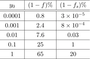
Table 3.1: Dependence of missing fraction and missing strength on the cutoff.
y0 (1−f)% (1−fs)%
0.0001 0.8 3×10⁻⁵
0.001 2.4 8×10⁻⁴
0.01 7.6 0.03
0.1 25 1
1 65 20
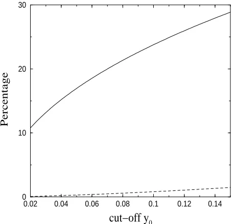
the strength is observed even if a large fraction of levels is missing. Table 3.1 lists 1−f
and 1−fs for various values of y0. For example, missing 25% of the levels corresponds to
missing only 1% of the strength. Fig. 3.1 shows 1−f and 1−fs as functions ofy0.
The next step is to calculate the average reduced width with the new strength and the new number of levels. Then one can recalculate the cut-off using a new average reduced width, recalculate 1−f and 1 −fs with the new cut-off, and then repeat the
entire process. This procedure is repeated until the missing fraction approaches a constant. Because the missing fraction is obtained with several iterations, this method is called the iterative method.
The procedure can be summarized as follows:
• First, the minimum reduced width γ2
min is determined from the data sequence. The
observed average reduced widthhγ2i
obs is determined with Eq. (3.4). • The dimensionless parametersyi are defined by
yi =
γi2
hγ2i
obs
, (3.8)
and y0 is determined from Eq. (3.5).
• The missing fraction of levels 1−f and the missing strength 1−fs are calculated
0.02 0.04 0.06 0.08 0.1 0.12 0.14
cut−off y
00 10 20 30
Percentage
Figure 3.1: The missing fraction (solid curve) and the missing strength (dashed curve) as functions of the cutoff parametery0.
• A new corrected number of levels in the sequence is determined from
Nnew =
Nobs
f , (3.9)
and the total strength is corrected
X
γi2 =
P
obsγi2
fs
. (3.10)
• These values are used to determine a new average reduced width
hγ2inew=
P
γi2 Nnew
. (3.11)
• Using this new average reduced width, a new value of y0 is defined, and the above
steps are repeated.
The corrected number of levels is
N = Nobs
f . (3.12)
One can then determine the average level spacingD or level densityρ from
D= 1
ρ =
Emax−Emin
N −1 . (3.13)
3.2
An example of the iterative method
As an example, we apply this method to 103 observed p +48Ti 1 2
+
resonances. The steps of the procedure described in the previous section are carried out as follows:
• The minimum reduced width of this sequence isγmin2 = 10 eV. The observed average reduced widthhγ2iobs = 426 eV is determined with Eq. (3.4).
• A y0= 0.023 and the reduced widths yi are found using Eqs. (3.8) and (3.5).
• A missing fraction 1−f = 0.117 and a missing strength 1−fs= 9×10⁻⁵are calculated
with Eqs. (3.6) and (3.7).
• A corrected number and total strength are found using Eqs. (3.9) and (3.10), respec-tively.
• With these values, a new average reduced width is determined from Eq. (3.11).
• A new cut-off is calculated with the value of hγ2i from the last step and the process
is repeated.
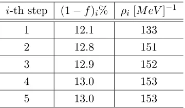
Table 3.2: Missing fraction for p +48Ti 1 2 +
resonances via the iterative method.
i-th step (1−f)i% ρi [M eV]−1
1 12.1 133
2 12.8 151
3 12.9 152
4 13.0 153
5 13.0 153
3.3
Advantages and disadvantages of the standard iterative
method
The iterative method is straightforward and easy to use. The main advantage of this method is the simplicity of its underlying assumption. Because of the absence of weak levels, the effect of the missing levels on the width distribution is systematic. With such a systematic effect, the formulation of the method is direct.
to quantify the uncertainty, an improved method is considered.
3.4
The maximum likelihood method
In order to determine the uncertainty in the missing fraction a modified Porter-Thomas distribution was introduced by Fr¨ohner [Fro80].
Pf(y) =
0 : y < y0
1 erfcµqy0/2
¶e
−y/2
p
2πy : y≥y0
(3.14)
This distribution goes to zero at values of y ≤ y0, reflecting the assumption that weak levels are not observed, and becomes the Porter-Thomas distribution when y ≥ y0. We will refer to this distribution as the truncated Porter-Thomas distribution. The truncated Porter-Thomas distribution is normalized to unity when integrated over y= [y0,∞[. With
this distribution one can construct the likelihood function
L=Y
i
p(yi). (3.15)
Implicitly in this expression, the average reduced width is a variable through
y= γ
2
hγ2i. (3.16)
The most likely value for the average reduced width will be the one that maximizes the likelihood function (3.15). The maximum condition gives
hγ2i=hγ2iobs
³
1 +
r
2y0 π
e−y0/2 erfcpy0/2
´−1
. (3.17)
The solution to this equation is the most likely value for the average reduced width hγ2i.
This equation can be solved iteratively starting from hγ2i ≈ hγ2iobs,where hγ2iobs is the
observed average reduced width. After substituting hγ2iobs forhγ2i in the y0 in the right
This procedure is repeated until “new” and “old” values ofhγ2iare sufficiently close. Again for most cases the iteration converges in about 5 steps. The resultinghγ2iis compared with the observed value in order to obtain 1−f, the fraction of levels missed.
The uncertainty inhγ2iis obtained by calculating the likelihood function as a func-tion ofhγ2i. The maximum of the likelihood function, or equivalently the maximum of the natural logarithm of the function, is located at the most likely value of hγ2i. The natural logarithm of the likelihood function is normalized to unity and the value of hγ2i where the normalized likelihood function (ln L)norm equals to one half of its maximum value is used
for a determination of the uncertainty in hγ2i, which in turn is used for the uncertainty inf. Applying this procedure to p +48Ti 1
2 +
resonances one obtainsf = 0.87+0−0..1311, which is in agreement with the standard method described earlier. These uncertainties are used to determine the uncertainty in the calculated number of levels, which will then give the uncertainty in the level density. For p +48Ti 1
2 +
resonances, the level density determined by this method is ρ= 153+32−30 MeV−1. The details of the analysis are discussed in chapter
6.
Spacing Analysis of Imperfect
Sequences
The spacings of a perfect GOE sequence are well approximated by the Wigner distribution. However, in practice the level sequence is almost always incomplete. One must then develop a new distribution that correctly describes the spacings of imperfect sequences. In the width analysis, the widths of the missing levels are systematically small, and therefore the width distribution for imperfect sequences was obtained by a simple modification to the Porter-Thomas distribution.
However, because the location of missing levels is random, the spacing analysis is much more complicated to formulate than the width analysis. Suppose that a fractionf of the totalN levels is observed and that a fraction (1−f) of the levels is missed at random. The spacing distribution is expressed in terms of a dimensionless spacing parameter – a spacing divided by the average spacing. It is convenient to consider 2 spacing parameters, (z ≡ Sobs/Dobs where Sobs is the observed spacing and Dobs is the observed average, and
x≡Sobs/DtruewhereDtrueis the “true” average). The relation between the two parameters
levels. With the variable x defined in this way, the functions P(k;x) are consistent with the notation in the literature.
An ansatz for the probability density function (PDF) for the spacings of an imperfect sequence was first introduced by Watsonet al. [Wat81a]. The probability PDF for observing a spacing x of the imperfect sequence was assumed to be
P(x) =p(0;x)f +p(1;x)f[1−f] +p(2;x)f[1−f]2+...
= ∞
X
k=0
f(1−f)kp(k;x), (4.1) wherex=Sobs/Dtrue.
In this chapter, a formal derivation of the PDF is provided as well as numerical examples.
4.1
Derivation of the PDF
The derivation of the Probability Density Function (PDF) for the spacings of im-perfect sequences can be performed as follows. The PDF can be written as
P(z) = ∞
X
k=0
akλp(k;λz), (4.2)
wherez=Sobs/Dobsandλis a parameter characterizing the incompleteness of the sequence.
Normalization conditions on the PDF are
Z ∞
0 P(z)dz = 1,
Z ∞
0 zP(z)dz = 1. (4.3)
The functionsp(k;λz) are the k-th nearest neighbor spacing distributions with normaliza-tions
Z ∞
0 p(k;λz)d(λz) = 1,
Z ∞
0 λzp(k, λz)d(λz) =k+ 1. (4.4)
Using the above normalization conditions, one obtains constraint equations for the coeffi-cients ak and the parameterλ:
∞
X
0
∞
X
0
ak(k+ 1) =λ.
To obtain these conditions one integrates both sides of equation (4.2)
Z ∞
0
P(z)dz= ∞ X k=0 ak Z ∞ 0
p(k;λz)d(λz) = 1, (4.6)
and
Z ∞
0 zP(z)dz =
∞
X
k=0 ak
Z ∞
0 zp(k;λz)d(λz), (4.7)
= 1 λ X k ak Z ∞
0 λzp(k;λz)d(λz) = 1.
In order to determine the coefficientsak an entropy is introduced,
S{ak}=−
∞
X
k=0
aklnak, (4.8)
along with two Lagrange multipliersαand β that correspond to the two constraints in Eq. (4.5). The variation of the entropy is then set to zero:
δ{−X
k
aklnak−α
X
k
ak−β
X
k
(k+ 1)ak}= 0. (4.9)
−X k
{δaklnak+δak+αδak+β(k+ 1)δak}= 0. (4.10)
Since the δak are linearly independent, each coefficient of δak should be zero and therefore
lnak+α+β(k+ 1) + 1 = 0⇒ak=e−α−1e−β(k+1). (4.11)
Applying the first constraint one obtains
X
ak= 1 =
X
e−α−1e−β(k+1) (4.12) = e−α−1Xe−β(k+1).
Substituting this into Eq. (4.11) yields
ak=
e−βk
P
One can simplify this further by using the identity
X
e−βk = ∞
X
k
(e−β)k= 1
1−e−β, (4.14)
which gives
ak = (1−e−β)e−βk. (4.15)
To obtain β one must use the second constraint equation.
λ=Xak(k+ 1) = 1 +
X
kak= 1 + (1−e−β)
X
ke−βk, (4.16)
where Eq. (4.15) was used in the second term. Writing each term in the sum as a total derivative leads to
X
ke−βk = −Xd(e−
βk)
dβ (4.17)
= − d
dβ
X
e−βk
= − d
dβ
³ 1
1−e−β
´
= e−
β
(1−e−β)2.
Thusλbecomes
λ= 1 + (1−e−β) e−
β
(1−e−β)2 =
1
1−e−β. (4.18)
One can show that the parameterλis just a rescaling parameter equal to the inverse of the observed fraction f. To show this, it is convenient to express the coefficients ak as
weighting factors that are explicitly connected with the functionsp(k;x). Theakcoefficients
can be written
ak=
Nk
N −m−1, (4.19)
where Nk is the number of spacings of type k (type k means there are k levels skipped),
For any incomplete sequence the following relationship holds:
N −1 =
kmax
X
k=0
(k+ 1)Nk. (4.20)
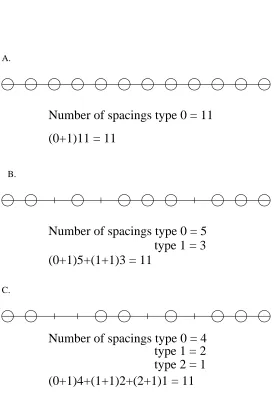
For example, when one level is missing between two levels, this reduces the number of spacings in the imperfect sequence by one. However, it will also increase the number of spacings of type k = 1 (type 1 because 1 level is skipped) by one. This is true for any number of levels missing. A diagram illustrating that the N −1 is conserved is shown in Fig. 4.1. Each circle represents a level, and each tick mark represents a missing circle, i.e., a missing level. There are 12 levels, and 11 spacings in the perfect sequence. Thus, the right hand side of Eq. (4.20) is always 11 forN = 12.
In part A of Fig. 4.1, there are 11 spacings of typek= 0, because no level is missing. Therefore N0 = 11. Substituting N0 = 11 in Eq. (4.20), (0 + 1)N0 = (0 + 1)11 = 11. In part B, there are 5 spacings of type 0, and 3 spacings of type 1. Therefore, N0 = 5, and
N1 = 3. Substituting in Eq. (4.20) gives (0 + 1)5 + (1 + 1)3 = 11. Similarly, in part C,
N0 = 4,N1 = 2, andN2 = 1 and therefore (0 + 1)4 + (1 + 1)2 + (2 + 1)1 = 11, which agrees
with Eq. (4.20).
Substituting Eq. (4.19) for the constraint equationλin Eq. (4.5), one obtains
λ=X(k+ 1)ak=
X (k+ 1)Nk
N−m−1. (4.21)
Using Eq. (4.20) this reduces to
λ= N −1
N −m−1 = 1
f, (4.22)
where
f = N −m−1
N −1 (4.23)
is of course the observed fraction of levels. The parameter λis equal to the inverse of f, and is simply a rescaling parameter.
Using Eq. (4.18) and λ= 1/f one can find β in terms off and substitute into Eq. (4.15) to obtain
A.
B.
C.
(0+1)5+(1+1)3 = 11
Number of spacings type 0 = 11
(0+1)11 = 11
Number of spacings type 0 = 4
(0+1)4+(1+1)2+(2+1)1 = 11
Number of spacings type 0 = 5
type 1 = 3
type 1 = 2
type 2 = 1
Finally substituting Eq. (4.24) and λ = 1/f in Eq. (4.2), and using x = z/f (note the Jacobian of the transformation fromz tox) one obtains
P(x) = ∞
X
k=0
f(1−f)kp(k;x). (4.25) This is the same as the ansatz in Eq. (4.1)
4.2
Theoretical GOE sequences
This section describes the numerical simulation of the Gaussian Orthogonal En-semble. We use the simulated GOE spectra to study various statistical properties. In this chapter we consider the nearest neighbor and thek-th nearest spacing distributions of both perfect and imperfect GOE sequences. In practice experimentally observed nuclear level sequences are almost always incomplete and therefore imperfect sequences are very important.
The entries of a real-symmetric GOE-matrix H are by definition Gaussian dis-tributed random numbers. The probability density distribution of the matrices is
p(H) =Cexp(−T rH
2
4σ2 ). (4.26)
For the non-diagonal entries
p(Hij) =
1
√
πσnd
exp(−H
2
ij
σ2
nd
), (4.27)
and for the diagonal entries
p(Hii) =
1
√πσ d
exp(− H
2
ii
σ2d), (4.28)
where the variances are given by
σnd= √
2σ, σd= 2σ. (4.29)
Since the distribution (4.26) is normalized,
Pij ≡
Z Hij
takes on values in the range [0,1]. Using distributions (4.27) and (4.28), one can write
Pij =
1
2(1 + erf(
Hij
σc
)), (4.31)
whereσc=σnd for the non-diagonal entries, andσc =σdfor the diagonal entries.
For a GOE matrix of size N ×N, one can generate N2 random numbers Pij for
i, j= 1, .., Nso that each of these numbers corresponds to an entry in the matrixH. In order to obtain values for entries of H, one must solve Eq. (4.31) for Hij. After diagonalization
of the matrix H, the diagonal elements E1 ≤ E2 ≤ · · · ≤ En form a GOE spectrum of
sizeN that obeys Wigner’s semicircle law. Alternatively, a more direct way is to generate Gaussian distributed random numbers for the entries of H and the eigenvalues of H will form a GOE spectrum. Since we are interested in constant level density, a spectrum larger than needed is calculated, and the central part of that spectrum is considered for further analysis. The size of the theoretical spectrum plays an important role because statistical variations will be smaller if there are many levels. Also, because of statistical fluctuations, a single sequence may not always display all GOE behavior. Instead, more reliable studies can be performed if statistical quantities are averaged over an ensemble of sequences.
Having generated theoretical GOE sequences, one can calculate various quantities from them and test or study their statistical properties. For example, one can draw a histogram of nearest neighbor spacings. To do that, one computes normalized spacings
xi =Si/D, whereSi =Ei+1−Ei, and the averageD=hSii= ∆E/(N−1), and then sorts
normalized spacings according to their size. A plot of the density of the nearest neighbor spacings (upper graph) and the cumulative density (lower graph) for 800 levels is shown in Fig. 4.2. Comparison with the Wigner surmise (dashed curve) shows a good fit. Obviously, the larger the number of levels, the closer (on average) the nearest neighbor distribution will approach the theoretical curve. One can generate a very large matrixH, say 105×105 and
0 1 2 3
x = S/D
0 0.2 0.4 0.6 0.8 1
∫
P(x)dx
0 0.2 0.4 0.6 0.8 1
P(x)
GOE spectrum N = 800
Wigner
0 1 2 3
x = S/D
0 0.2 0.4 0.6 0.8
10 1 2 3
0 0.2 0.4 0.6 0.8 1
P(x)
800 levels
220,000 levels
Figure 4.3: The histogram for the nearest neighbor spacing distribution is much closer to the Wigner distribution (solid curve) for 220,000 spacings (lower graph) than for 800 levels (upper graph).
4.3
The
k
-th nearest neighbor spacing distributions
The probability density function (4.1) for the spacings of the imperfect GOE se-quences is a weighted summation of thek-th nearest spacing distributionsp(k;x). Thek-th nearest neighbor probability functionp(k;x) gives the probability for a normalized spacing
x between two levels, given that there are k levels between the two. A closely related set of functions are theE(k;x), which give the probability that a randomly chosen interval of length x contains exactly k levels. Numerical values for E(k;x) and recursive analytical formulae for E(k;x) are given in [Meh91]. Thep(k;x)’s and theE(k;x)’s are related by a simple recursion formula
p(k;x) =
k
X
j=0
(k−j+ 1) d
2
dx2E(j;x). (4.32)
Thus, in principle, the spacing distributionp(k;x) for any order of kcan be found in terms of the functionsE(k;x). For k= 0,
p(0;x) = d
2
dx2E(0;x), (4.33)
reduces to the Wigner distribution. If a single level is missed, ak = 1 spacing is observed and the probability function is the next nearest spacing distribution
p(1;x) = d
2
dx2E(1;x) + 2p(0;x). (4.34)
When two consecutive levels are missed, ak= 2 spacing is observed and the corresponding probability function is
p(2;x) = d
2
dx2E(2;x) + 2p(1;x)−p(0;x). (4.35)
0 2 4 6
x = S/D
0 0.2 0.4 0.6
P(x)
k = 1
0 2 4 6
k = 2
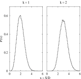
Figure 4.4: k = 1 and k = 2 nearest neighbor spacing distributions. The histograms are calculated using computer generated sequences and the dashed curves are interpolations.
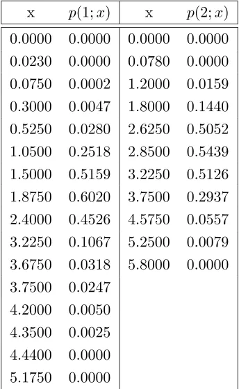
Gaussian orthogonal spectra of size 110 was generated and the k = 1 and k = 2 nearest neighbor spacings histograms were calculated for a total of 330,000 levels. The results are shown in Fig. 4.4 where the dashed line for k= 1 is a result of a polynomial interpolation and fork= 2 a rational function interpolation. Values for the functionsp(1;x) andp(2;x) at various points are given in Table 4.1. With these values, one can interpolate (for instance, using subroutine ratint in [Pre92]) the functions p(1;x) and p(2;x) for any x without having to calculate the second derivatives forE(1;x) and E(2;x).
Table 4.1: Calculated values forp(1;x) and p(2;x). x p(1;x) x p(2;x)
0.0000 0.0000 0.0000 0.0000 0.0230 0.0000 0.0780 0.0000 0.0750 0.0002 1.2000 0.0159 0.3000 0.0047 1.8000 0.1440 0.5250 0.0280 2.6250 0.5052 1.0500 0.2518 2.8500 0.5439 1.5000 0.5159 3.2250 0.5126 1.8750 0.6020 3.7500 0.2937 2.4000 0.4526 4.5750 0.0557 3.2250 0.1067 5.2500 0.0079 3.6750 0.0318 5.8000 0.0000 3.7500 0.0247
0 2 4 6
x = S/D
0 0.2 0.4 0.6
P(x)
k = 1
0 2 4 6
k = 2
Figure 4.5: k = 1 and k = 2 nearest neighbor spacing distributions. A solid curve is the Gaussian approximation while a dashed line is an interpolation to the numerically generated
p(k;x).
by Frenchet al. [Fre78] to be approximately
σk2 = 1
πln(2π[k+ 1] +γ+ 1)−
5
12, (4.36)
where γ = 0.577, Euler’s constant. In fact, this approximation is fairly close even for
k = 1, 2 as shown in Fig. 4.5. The difference between using the interpolations and the Gaussian approximation in the calculation of the PDF is small. The k-th nearest spacing distribution functions p(k;x) are used in constructing a probability density function that will be applied to data sets in this work.
In summary, p(0;x) is the Wigner distribution, higher order spacing distributions
approxi-mated by Gaussians whose variance is given by Eq. (4.36) and centered atk+ 1.
4.4
Spacing distributions for imperfect GOE sequences
Once the p(k;x) functions are available, the Probability Density Function (PDF) for the spacing between two observed levels can be obtained with Eq. (4.1). In practice the summation is truncated at a value of k ≥xmax+ 1 wherexmax is the largest spacing
of interest. Suppose, for example, that the largest spacing is x = 3 (from the Wigner distribution, the probability of a spacing greater than x = 3 is 0.1%, see Table 6.2). As shown in Fig. 4.6, the spacing probabilities for k ≥ 5 are very small when xmax = 3.
Therefore in this case the sum overk in Eq. (4.1) will include only termsk≤4.
To test Eq. (4.1), one can generate incomplete GOE sequences with a certain fractionf of the total levels observed, and a fraction 1−f of levels missed randomly. GOE sequences ofN levels are generated in the same fashion as discussed earlier and a fraction 1−f of these levels is removed randomly. The resulting sequences will be imperfect GOE sequences with a missing fraction 1−f. As an example, consider an ensemble of 3000 GOE sequences of size N = 70, i.e., 210,000 levels. The nearest neighbor spacing distributions for f = 0.80, f = 0.65, and f = 0.50 are plotted in Fig. 4.7. The solid curves are Eq. (4.1) for the respective values of f and the dashed curve is the Wigner distribution. The deviation of the histogram calculated from the simulated data from the Wigner distribution increases with the increasing missing fraction. On the other hand, the PDF given by Eq. (4.1) describes the spacings of incomplete sequences very well.
To obtain a quantitative test, one can use the maximum likelihood method. First, one needs to calculate the likelihood function
L=Y
i
P(xi, f), (4.37)
0
2
4
6
x = S/D
0
0.2
0.4
0.6
0.8
P(x)
Wigner
k = 1
k = 2
k = 3
k = 4
x
maxFigure 4.6: The summation over k in Eq. (4.1) can be truncated at k = 4 if xmax = 3
0
1
2
3
4
x= S/D
0
0.2
0.4
0.6
0.8
1
P(x)
f =1 (Wigner)
f = 0.8
f = 0.65
f = 0.5
0.8
0.82
0.84
0.86
0.88
0.9
f
0
0.5
1
(ln
L)
norm
0
1
2
3
4
x = S/D
0
0.2
0.4
0.6
0.8
1
P(x)
Figure 4.8: NNSD forN = 3300 spacings of an imperfect GOE for f = 0.85 is shown in the upper graph. The likelihood function has a maximum at f = 0.848±0.018.
runs through all spacings. Evaluating lnLinstead is often easier
lnL=X
i
lnP(xi, f). (4.38)
The most likely value of f is the value that maximizes the likelihood function (4.38). The natural logarithm of the likelihood function is normalized to unity and the uncertainty inf
0.8 0.85 0.9
f
0 0.5 1(ln
L)
norm0 2 4
x = S/D
0 0.2 0.4 0.6 0.8 1
P(x)
0.8 0.85 0.9
f
0 0.5 1
0 2 4
x = S/D
0 0.2 0.4 0.6 0.8 1
N = 1000
N = 3300
Figure 4.9: The likelihood function for a larger number of spacings provides a better estimate of f.
Experimental Methods
In the study of level densities using nuclear resonances there are several important considerations. There are both advantages and disadvantages in using proton or neutron resonances for level density studies. Some of these are discussed in this chapter. A major difference in neutron and proton induced reactions is the difference in penetrability due to the effects of the Coulomb barrier. Because of this and other differences, the proton and neutron resonances must be treated differently.
One of the basic requirements that apply to both proton and neutron resonances is that in order for a sequence to be suitable for statistical analysis, the size of the sequence should be as large as possible. If the number of levels is too small then statistical properties determined using that sequence will have a low confidence level. An approximate lower limit is taken to be 25. Since the fractional statistical error in a GOE sequence ofN levels isq0N.27 [Lyn68],N = 25 corresponds to an approximately 10% relative error.
5.1
Proton resonances
angular momentum is not too large one can see resonances with several different l values. This is advantageous because differentlvalues are needed for the study of parity dependence of the level densities. Thus proton resonances are good candidates for the study of the parity dependence of level densities.
The equipment and experimental procedures used in the proton scattering measure-ments are described in [Wat80, Smi89, Li90] and will not be discussed here. The general procedure to obtain the spin and parity of resonances is described below. A detailed descrip-tion can be found in [Wat80, Smi89, Li90]. The strong Coulomb interference effect leads to easily identifiable characteristic shapes at different angles for resonances of different orbital angular momentum l. Proton resonance parameters are obtained from the experimental data by fitting the data using the multi-level multi-channel reaction code MULTI, first written by Sellin [Sel69] and extended and revised over the years by various authors. The code is based on the R-matrix theory by Lane and Thomas [Lan58].
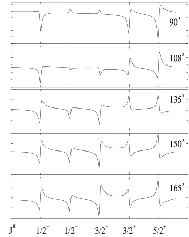
The spin and parity of the resonance is determined by shape analysis, i.e., the line shape of the resonance is a function of spin, parity, and the scattering angle. To illustrate, Fig. 5.1 shows the shapes of hypothetical resonances for variousJπ at five detector angles in elastic scattering. In this fictitious example, the resonance width is fixed so that the shape change is only due to difference in Jπ and angle [Bea02]. Since the highest value of Jπ in the data analyzed in this dissertation is 5/2+, the discussion will be limited to
d
σ
/d
Ω
arbitrary units
1/2
+1/2
−3/2
−3/2
+5/2
+J
π
90
o108
o135
o150
o165
odifference is small for weak resonances. Sometimes inelastic scattering measurements can be used to distinguish the different J values. The two resonances appear similar in the elastic channel and are difficult to distinguish, but due to the anisotropy in the inelastic channel the resonance often can be uniquely assigned a J value. However, there are cases when one cannot distinguish between two choices. Although this ambiguity is limited to a relatively few resonances, it can have a large effect on the level densities. A fundamental difficulty with proton resonances is that the data are limited to the light and medium mass regions. In light nuclei, poor statistics limit the application. Therefore proton resonances primarily provide good data in the medium mass region.
As a summary, proton resonances are suitable for the study of parity and angular momentum dependences of nuclear level densities in medium mass nuclei because of the availability of resonance sequences with various spins and parities.
5.2
Neutron resonances
A key difference between neutron and proton resonances is that there are many fewer neutron resonances observed with a higher l value. Because at low energies the penetrability difference is large betweens-wave andp-wave neutron resonances, most of the stronger resonances ares-wave and most of the weaker resonances are p-wave. Since there are fewer resonances with a higherlvalue, neutron resonances seem less suitable for a study of parity and spin dependence of level densities than are proton resonances.
the Porter-Thomas distribution for neutron widths.
The Bayesian conditional probability of a resonance beingp-wave is [Mit01]
BP(l= 1|gΓn) =
P1P(gΓn|l= 1)
P1P(gΓn|l= 1) +P0P(gΓn|l= 0)
(5.1)
where P0 and P1 are a priori probabilities for the resonance to be s- or p-wave, Γn is the
neutron width and g is the statistical factor. P(gΓn|l = 0) and P(gΓn|l = 1) are the
Porter-Thomas probabilities for a givengΓnvalue andl= 0 or 1. The Bayesian conditional
probability is further expressed in terms of average resonance parameters such as level spacings and strength functions. Using this method, one can determine the l value of the resonances with reasonable confidence.
Analysis of Resonance Data
6.1
Introduction
The analysis of resonance data is performed using the two methods that have been described in previous chapters: width analysis and spacing analysis. As discussed earlier, in analyzing experimental data one must consider effects of missing levels, non-statistical ef-fects, and spin misassignment issues. These topics are considered below for the two analysis methods.
6.2
Missing levels
6.2.1 Width analysis
An improved iterative method for the width analysis to determine the observed fraction of levels was described in chapter 3. In this section the method is applied to p+48Ti
s-wave resonances. There are 103 observeds-wave resonances. The smallest reduced width is γ2min = 10 eV and the observed average reduced width is hγ2iobs = 426 eV. Recall that
the maximum likelihood condition gives
hγ2i³1 +
r
2y0 π
e−y0/2 erfcpy0/2
´
Substituting hγ2iobs = 426 eV and y0 = γ
2
min
hγ2i
obs = 0.023 gives the next value of hγ
2i
1 = 374
eV. Using this new average reduced width hγ2i1 = 374 eV, one can define a new cut-off y0new = 0.027 and repeat the above steps until convergence is achieved. The result is hγ2i = 370 eV, which corresponds to an observed fraction f = 0.87. To determine the uncertainty inf the likelihood function is evaluated with Eq. (3.15) and the result is shown in Fig. 6.1. The maximum of the likelihood function is located atf = 0.87. The uncertainty inf is obtained by locating the value off where the (normalized) natural logarithm of the likelihood function is 0.5 of its maximum value. As shown in Figure 6.1, the uncertainties are ∆−= 0.11 and ∆+= 0.13. Therefore the fraction observed for p +48Ti 12+ resonances
is f = 0.87+0−0..1311. These uncertainties can be used for determining the uncertainty in the calculated number of levels, which provides the uncertainty in the level density.
A comparison of the truncated Porter-Thomas distribution and the data is given in Fig. 6.2. Note that the data is truncated at the low side, indicating the absence of small widths. A comparison with the cumulative probability is presented, and it also indicates that small widths are missed.
This method is reliable when the data set is pure. When there are non-statistical effects such as analog states, one must exclude those resonances from the sequence before applying this method. To illustrate how analog states can affect the sequence, consider an example of 35 observed 12−resonances in p +56Fe. In Fig. 6.3 there is a peak at a large value
ofy. This peak is due to the strong analog state at Ep = 3.958 MeV. Because of this strong
non-statistical effect, the cumulative distribution appears to agree well with the cumulative number of levels, as if most levels were observed. Moreover, the iterative method will give false results because the observed average reduced width ishγ2iobs = 2358 eV, much larger
than the one calculated after analog states are removed, hγ2iobs = 1065 eV. The calculated
0.6
0.7
0.8
0.9
1
f
0
0.5
1
(ln
L)
norm
p +
48Ti, J
π= 1/2
+f = 0.87
−
∆
f = 0.11
+
∆
f = 0.13
Figure 6.1: Maximum likelihood function for p +48Ti 1 2
+
0.01 0.1 1 10
y =
γ
2/ <γ
2>
0.01 0.1 1
y
1/2
P(y)
0 0.2 0.4 0.6 0.8 1
∫
P(y)dy
p +
48Ti, J
π= 1/2
+Figure 6.2: Reduced width distribution for p +48Ti 1 2 +
analysis is applied.
6.2.2 Spacing analysis
The theoretical distributions for the spacings and the maximum likelihood method to estimate the observed fractionf of imperfect GOE sequences were presented in chapter 4. In this section the method is applied to p +48Ti 1
2 +
resonance spacings and the results are compared with the results of the width analysis obtained in the previous section. There are Nobs =103 observed 12+ resonances, and therefore 102 spacings. The observed average
spacingDobs is simply
Dobs =
∆E Nobs−1
= 3.8574−3.0850
102 MeV = 7.6 keV. (6.2)
Before applying the spacing analysis to proton resonances, one should unfold the energy dependence of the level density. The level density increases exponentially with in-creasing incident particle energy. When the energy interval under consideration is significant compared with the compound nuclear excitation energy, the change in the level density must be unfolded. The unfolding is performed for proton resonances before the spacing analysis is applied. For neutron resonances, the incident neutron energy range is very small and the level density increase is negligible. Thus the unfolding is not used for neutron resonances.
A simple procedure is to average the density over a few adjacent spacings and fit to the constant temperature form of the level density
ρ(E) = 1
D =ρe
(E/T), (6.3)
or equivalently to a linear function lnD = a+bE. The slope of the fit gives b = −1/T. Then a new sequence of levels is generated
Enew =Emin+ (Emax−Emin)
e(E−Emin)/T −1
e(Emax−Emin)/T + 1. (6.4)
0.01 0.1 1 10
y =
γ
2/ <γ
2>
0.01 0.1 1
y
1/2
P(y)
0 0.2 0.4 0.6 0.8 1
∫
P(y)dy
p +
56Fe, J
π= 1/2
−0.01 0.1 1 10
y =
γ
2/<γ
2>
0.01 0.1 1
y
1/2
P(y)
0 0.2 0.4 0.6 0.8 1
∫
P(y)dy
p +
56Fe, J
π= 1/2
−sequence, then a more sensitive procedure is needed. Such a procedure is described in [Shr90] and is applied to all proton sequences considered in this work. In this approach, the integral ofρ(E)
N(E) =
Z E
0
ρ(E)dE= exp(E−E0/T)−exp(−E0/T) +N0 (6.5)
is used. Once the best fit toN(E) was obtained a new sequence was generated
Enew =Emin+ (Emax−Emin)
F(E)−F(Emin)
F(Emax)−F(Emin)
, (6.6)
whereF(E) denotes the best fit toN(E).
The endpoints of the energy interval Emin and Emax do not change under this
transformation. An example to illustrate the difference between the observed and the unfolded sequences is shown in Fig. 6.5 for p +48Ti 1
2 +
resonances. The temperature for this example isT = 0.8 MeV. Note that here the term temperature is not used in the usual nuclear sense. This temperature is specific to each sequence, while usually the nuclear temperature applies to a given nucleus. Here temperature is a parameter related to a purely empirical fit. The spacing analysis was performed with the unfolded sequence.
Before applying the theoretical distribution to the sequence, a qualitative evaluation of the data can be made. First, by looking for anomalously large spacings, one can estimate whether a large fraction of levels is missing from the sequence. Listed in Table 6.1 are 3 pairs of levels with spacings that are more than 2.5 times larger than the average spacing. Values ofx are shown in the upper graph in Fig. 6.6.
Table 6.1: Large spacing anomalies in p +48Ti 12+ resonances.
index x=S/D Energy interval [MeV]
x1 2.9 3.2220-3.2490
x2 2.6 3.3613-3.3826
x3 3.0 3.5820-3.7302
Table 6.2: Percentage of levels with spacings ≥x.
x= DS % of levels≥x
1.95 5 %
2.23 2 %
2.42 1 %
0
25
50
75
100
Level index
0
5
10
15
20
1/x
0
1
2
3
x
p +
48Ti, J
π= 1/2
+, Ν = 103
x1
x2
x3
y1
y2
y3
y4
x= DS change with the changing average spacingD=Dobsf becausef changes. Therefore
the histogram is different for each value of f. As can be seen from Fig. 6.7, the histogram for f = 0.87 (the value suggested by the width analysis), is closer to the PDF than the other two cases. Although such a visual inspection is useful, clearly one needs more precise results. Thus the maximum likelihood method is used to determine the most likely value of f by varying f and calculating the likelihood function given by
lnL(f) =X
i
lnP(xi). (6.7)
whereP(xi) is given by Eq. (4.1). The result is shown in Fig. 6.8.
One must be cautious in evaluating ln L for samples of this size. Because of the change in histograms with changing f, lnL fluctuates. Therefore some averaging is neces-sary to reduce the fluctuation. Terms inPilnP(xi) that correspond to the same bin in the
histogram are grouped together. Then we assume that the PDF for spacings that belong to the same histogram is approximately equal, i.e., that the PDF can be evaluated at the midpoint of each bin and multiplied by the number of spacings in that bin. For example, in Eq. (6.8) suppose there are n1 spacings in the first bin. Since these spacings are in the
same bin they are close in value. Thus the sum of the PDF evaluated at each of these n1
spacings can be approximated by the PDF evaluated at the center point xmid of the bin
times the number of spacings in that bin, n1.
X
i
lnP(xi) = lnP(x1) + lnP(x2) +...+ lnP(xn1)
| {z }
n1lnP(xmid)
+· · ·. (6.8)
The same applies for all the other bins, resulting in
lnL=n1lnP(xbin1) +n2lnP(xbin2) +· · ·+nbinNlnP(xbinbinN). (6.9)