A Method of Predicting Composite Magnetic Sources Employing Particle Swarm Optimization

(1)

A Method of Predicting Composite Magnetic Sources Employing

Particle Swarm Optimization

Sotirios Spantideas, Nicolas Kapsalis, Sarantis Dimitrios Kakarakis, and Christos Capsalis

Abstract—In this paper, the problem of predicting the parameters (positions and magnetic moments) of an Equipment Under Test (EUT) composed of a magnetic dipole and quadrupole is studied. Firstly, a multiple magnetic dipole and quadrupole model (MDQM) is developed to simulate the magnetic behavior of the EUT. The parameters of the model are calculated using the values of the near field measurements applying the Particle Swarm Optimization (PSO) algorithm. For the evaluation of the method, extended simulations were conducted, producing theoretical values and distorting them with noise, and then the developed algorithm was used to create the proper MDQM. As an evaluation criterion, the relative difference between the theoretical and the MDQM’s magnetic field is considered.

1. INTRODUCTION

The problem of finding the magnetic signature of any Equipment Under Test (EUT) is crucial in many applications and has been thoroughly discussed [1–5]. Magnetic cleanliness is one of the most important applications employing the magnetic behavior of EUTs. Since space missions intending to measure planetary magnetic fields operate in great distances from planets, the measuring devices of the spacecrafts must be placed in “magnetically clean” specification points, namely where the magnetic field of the spacecraft is kept below certain thresholds, i.e., between 0.1–1 nT [1].

In order to facilitate the determination of “magnetically clean” specification points, a plethora of approaches has been proposed [6–9]. The predominant approach employs the development of multiple magnetic dipole models (MDMs), which emulates the magnetic field of EUTs. Based on near-field measurements in coil facilities and employing deterministic [1–5] or stochastic methods, the parameters of the equivalent MDM (position and magnetic torque) may be estimated. The MDM technique has been employed in many applications such as near field analysis in the antennas field [10], electrocardiography simulation [11] and the representation of electromagnetic emissions of an Integrated Circuit [12]. Furthermore, source reconstruction methods based on near field measurements have been addressed in the literature [13, 14].

Although the MDM can predict the magnetic behavior of an EUT [15], quadrupoles’ magnetic fields are not taken into account. Hence, the accuracy of the resulting model may be further enhanced by combining dipoles and quadrupoles in a single Multiple Dipole and Quadrupole Model (MDQM). Modeling the magnetic behavior of this combination is quite challenging, since the magnetic field produced by quadrupoles is significantly weaker than this produced by dipoles. Furthermore, in numerous cases, namely in cases when the quadrupole is positioned near the dipole, it may be classified as noise. The efficient modeling of an MDQM is quite important in applications that use permanent magnets for calibration purposes, since these magnets may include higher order terms, like quadrupole and octupole terms. Moreover, the MDQM prediction may allow post — processing removal of the

Received 29 September 2014, Accepted 6 November 2014, Scheduled 12 November 2014

(2)

quadrupole magnetic ﬁeld from a set of measurements. Finally, the proposed method allows prediction of an EUT’s magnetic behavior in distances where the ambient noise is comparable to the quadrupole’s magnetic ﬁeld.

An alternative to deterministic methods, stochastic or metaheuristic methods, has become recently available to efficiently find global optima in NP — hard optimization problems. In [16, 17] such metaheuristic methods have been employed to study electromagnetic radiation problems. A main advantage of metaheuristic search techniques is the fact that they do not depend on a correct assumption of a starting point. Furthermore, they do not need any assumption on the objective function’s properties. As a result, they are more robust compared to deterministic methods. Due to the high number of function evaluations needed to define the global optimum, increased computer power is necessary. One of the most recently developed stochastic methods, imitating natural phenomena, i.e., the movement of bees inside a field, is Particle Swarm Optimization (PSO) [18]. PSO has been used in a variety of problems, such as antenna design ([16, 17]) and resource allocation [19].

In the present work a PSO approach is employed to calculate the parameters of an MDQM creating a magnetic field equivalent to a set of simulated measurements. PSO is selected in the present work, since the authors found out that the Genetic Algorithms (GAs) are not able to predict the magnetic field of a quadrupole treating it as a single dipole. In order to evaluate the proposed method, initially a theoretical model — composed by a magnetic dipole and quadrupole randomly positioned — is assumed. The aforementioned model may be regarded as a simulated EUT. The magnetic field values of this model in certain locations (observation points) are then produced. The observation points selected in the present work are located at a circle centered to the assumed EUT to be modeled. This results in the calculation of the theoretical values of the simulated measurements.

Additionally, in order to evaluate the denoising capabilities of the proposed method the theoretical values are distorted with noise in order to create a set of simulated with a maximum predeﬁned percentage of distortion (5%). These simulated measurements are then used to predict the combination of dipole’s and quadrupole’s positions and magnetic moments. The paper is organized as follows: Section 2 includes the theoretical background, while in Section 3 the numerical results are presented followed by the conclusions of the process.

2. PSO: A SHORT OVERVIEW

PSO is a stochastic evolutionary computation technique and it is inspired by the synchronized movement of swarms. It was developed in 1995 by Kennedy and Eberhart [18] and imitates the movement of bees (particles) across a field. Particles represent each individual in the swarm. They may be viewed as a member of the population. All particles start from random locations (during the initialization phase) and move towards the directions of (i) personal and (ii) global optimum. The particles’ ultimate target is to locate the spot with the maximum concentration of pollen (global optimum) in a given field (search space). During the initialization phase, the particles begin their movement in random points with random velocities (vectors denoting direction and speed towards updated positions). In every iteration, the particles move to new positions (locations of each particle inside the search space) according to their updated velocities. The updated velocities take into account both (i) the particle’s personal (the fittest vector encountered by each particle) and (ii) the swarm’s global optimum (the fittest vector (positions and moments) encountered by all particles). The particles’ velocities depend on whether exploration of the search space (represented by personal best) or the exploitation of the possible global optimum is predominant. The above two opposite targets are quantified in the model by the use of two factors. As PSO unfolds and the particles explore the search space, both global and personal optima may be updated, resulting in new velocities. After a predefined number of iterations, PSO finalizes and converges to a possible global optimum.

3. MATHEMATICAL FORMULATION

The EUT’s magnetic behavior is modeled by a set of 1 magnetic dipole and 1 magnetic quadrupole. The dipole is positioned at (x_d, y_d, z_d), and the respective magnetic moment is calculated as follows:

(3)

Accordingly, M observation points, positioned at (x0j, y0j, z0j), j = 1,2, . . . , M, are considered. The

magnetic ﬁeld of the dipole at the observation pointjis expressed as the superposition of its components:

B_dj = μ0 4·π ·

3·m_d·ρ_dj·( ˆm_dj ·ρˆ_dj) ρ3

dj

−md

ρ3

dj

(2)

where

ρ_dj =

(x0j −xd)2+ (y0j−yd)2+ (z0j −zd)2 (3)

The magnetic ﬁeld of the dipole in observation pointj is then calculated via

B_d=

N

i=1

B_x

dj ·xˆ+

N

i=1

B_y

dj ·yˆ+

N

i=1

B_z

dj ·zˆ (4)

The magnetic ﬁeld of a linear quadrupole in observation pointj can be calculated via [20]

B_qj = μ0 4·π ·

3·m_q 4·ρ4

qj

·5·( ˆm_q·ρˆ)2−1

ˆ ρ

−3·mq

2·ρ4

qj

·( ˆm_q·ρˆ) ˆm_q

(5)

wherem_q is the quadrupole magnetic moment and

ρ_qj =

(x0j −xq)2+ (y0j −yq)2+ (z0j−zq)2 (6)

The magnetic ﬁeld of quadrupole in observation point j is then calculated as the superposition of the magnetic ﬁelds of two linear quadrupoles perpendicular to each other [20].

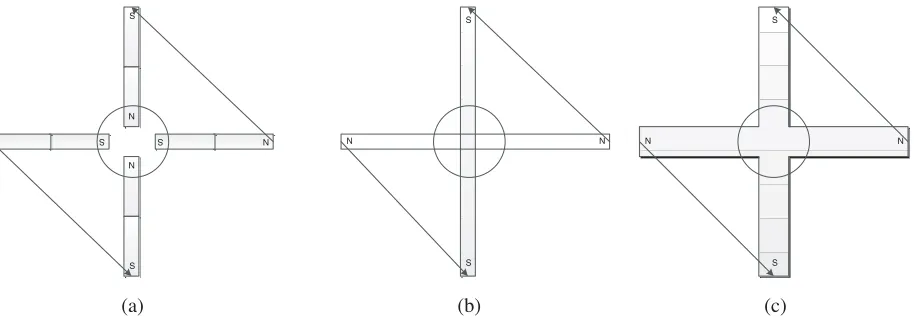
In Fig. 1(a) four dipoles in close proximity with equal magnetic moments’ magnitude are presented. The poles inside the circle (two South and two North) are approximately neutralized. Evidently, the aforementioned conﬁguration may be considered equivalent as two linear quadrupoles forming a normal quadrupole [20] (Fig. 1(c)).

S

N

S

N S N

N

S

N N

S

N N

S

(a) (b) (c)

Figure 1. Array of (a) 4 dipoles (b) 2 linear quadrupoles perpendicular to each other and (c) a normal quadrupole producing equivalent magnetic ﬁelds.

Another equivalent conﬁguration composing of two dipoles in close proximity — ε, where ε is a small number — with opposite dipole magnetic moments is depicted in Fig. 1(b). As shown in [20] the quadrupole’s magnetic moment is proportional to the product ofε and dipole’s magnetic moment. For example, two dipoles with magnetic moments 30 mAm2 _and ₋_{30 mAm}2 _{respectively, separated by}

0.7 cm may be considered as a quadrupole with magnetic moment m_q≈0.15 mAm3_.

(4)

is represented by a (1 ×6) vector. Additionally, the quadrupole is deﬁned by a reference dipole (x_q, y_q, z_q, m_x_q, m_y_q, m_z_q) and a dipole in close proximity with opposite magnetic moments represented by (x_q+ε_x, y_q+ε_y, z_q+ε_z,−m_x_q,−m_y_q,−m_z_q), where

ε=

ε2

x+ε2y +ε2z (7)

The proposed scheme determines the positions and magnetic moments of the dipole and the reference dipole of the MDQM. As a result, every particle is represented by a (1×12) vector E. Its elements, e_i, represent the positions and magnetic moments of the dipoles. Evidently, the variable values that minimize the objective function need to be determined.

4. APPLYING PSO FOR THE MDQM PROBLEM

To formulate the MDQM problem, a (3×M) matrixTBth, containing the theoretical magnetic field values, is introduced. Each line of TBth corresponds to the magnetic field components B_x, B_y, B_z at the observation pointj= 1,2, . . . , M. Accordingly, a (3×M) matrixTBis employed in order to include the magnetic field produced at every iteration. After the evaluation of pbest and gbest, the particles’ new velocities are calculated via (8) [18].

u_i,n=w·u_i,n+c1·rand()·(pbesti,n−pi,n) +c2·rand()·(gbesti,n−pi,n) (8)

where w denotes the weight of the previous iteration’s velocity, and c1, c2 are factors determining the

tradeoﬀ between exploring the search space and exploiting the possible optimal solution. Finally, p_i,n stands for the position of element iof agent n, n= 1,2, . . . , N. In the present work, c1 =c2 = 2 and

w= 0.5.

Afterwards, the agents’ new positions are calculated as follows:

p_i,n=p_i,n+u_i,n (9)

As the proposed scheme unfolds, each agent updates its position and velocity (8)–(9), and then Equations (1)–(10) are used to updateTB. Two matricesTBpandTBgare introduced to contain the magnetic ﬁeld values corresponding topbest and gbest, respectively.

Finally, to quantify the quality of each solution — represented by each agent — is deﬁned as follows:

F =

3

i=1

M

j=1

(T Bg_i,j−T Bth_i,j)2 (10)

At every iteration the ﬁtness function is calculated for all agents. In case that the ﬁtness function’s value of the updated position of agentnis lower compared to the corresponding value ofpbest (orgbest),

pbest (or gbest) is replaced by the former. The ﬂowchart of the proposed scheme is depicted in Fig. 2.

Evidently,F is nulliﬁed if TBgand TBth are equal, stemming from models with equal parameters.

5. SIMULATION RESULTS

In this section the efficiency of the proposed scheme is evaluated when predicting an MDQM, employing theoretical magnetic field values (Case A) and distorted by maximum 5% (Case B). Since the quadrupole’s contribution to the total magnetic field vanishes as the observation distance increases, the measurement points are chosen to form a circle of 40 cm radius. Moreover, in both casesε= 0.7 cm.

5.1. Case A

A set composing of one dipole and one quadrupole was employed to create a magnetic ﬁeld in various points. The aforementioned ﬁeld’s values were created via Equations (1)–(10) and were included in

(5)

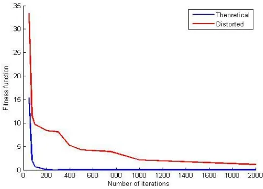
Figure 2. Convergence of the proposed scheme with respect to the number of iterations when the theoretical (blue line) or distorted values (red line) are employed.

Table 1. Initial parameters of the dipoles.

x (cm) y (cm) z (cm) m_x (mAm2) m_y (mAm2) m_z (mAm2)

Dipole 0 0 0 0 0 30

Reference dipole of quadrupole

−0.35 0 −1 −10 −10 0

Dipole 2 of

quadrupole 0.35 0 −1 10 10 0

Table 2. Parameters of the MDQM.

Dipole 0.0005 0.0000 0.0000 0.0001 −0.0000 30.0000

−0.3500 −0.0000 −1.0000 −10.0000 −10.0000 0.0217

Dipole 2 of

quadrupole 0.3500 −0.0000 −1.0000 10.0000 10.0000 −0.0217

The proposed scheme converges to the MDQM whose parameters are given in Table 2, minimizing the ﬁtness function value toF = 9.6439·10−9. Evidently, PSO was able to reconstruct almost identically the theoretical model, distinguishing the dipole’s and quadrupole’s contributions to the magnetic ﬁeld, despite their close proximity.

(6)

Dipole 10 10 10 0 0 30

−0.35 0 −1 −10 −10 0

Dipole 2 of

quadrupole 0.35 0 −1 10 10 0

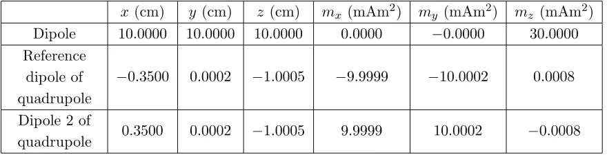
Table 4. Parameters of the MDQM using PSO.

x (cm) y (cm) z(cm) m_x (mAm2₎ _m

y (mAm2) mz (mAm2)

Dipole 10.0000 10.0000 10.0000 0.0000 −0.0000 30.0000 Reference

dipole of quadrupole

−0.3500 0.0002 −1.0005 −9.9999 −10.0002 0.0008

Dipole 2 of

quadrupole 0.3500 0.0002 −1.0005 9.9999 10.0002 −0.0008

From the above veriﬁcation cases, it is established that the presented method is able to identify the existence of the quadrupole regardless of its distance from the dipole and precisely predict the model’s parameters.

In Fig. 2 the ﬁtness function with respect to the number of iterations is shown.

5.2. Case B

In order to verify the ability of the algorithm to accurate predict the MDQM, a dipole with magnetic moment (0, 0, 30) mAm2 and a quadrupole composed of two dipoles are used as EUT. The reference dipole of the quadrupole has magnetic moment (−10, −10, 0) mAm2. The positions of the dipole and the reference dipole of the quadrupole were drawn from a Normal distribution with mean μ= 0 and standard deviation σ = 1. Ten diﬀerent EUTs were created. For every EUT, a TBth matrix was created, where the magnetic ﬁeld values, calculated from Equations (1)–(10), are included. These

TBth matrices were used as input to the algorithm.

In Fig. 3 the theoretical and the MDQM positions, for all ten EUTs, are presented in 2-D at thexy, xz andyz planes. More explicitly, the blue cross “+” represents the theoretical position of the dipoles, the blue “×” represents the theoretical position of the quadrupoles, composed of two dipoles, and the red dot “·” and circle “◦” represent the MDQM predicted positions of the dipoles and the quadrupoles, respectively.

From Fig. 3 it is readily observed that, the proposed scheme accurately predicted the theoretical EUTs.

5.3. Case C

(7)

(a)

(c) (b)

(8)

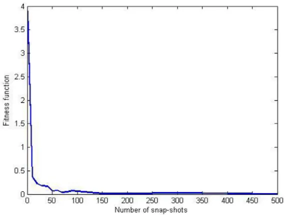
denoising method TBth values are replaced by the average of several distorted measurements, i.e., snap-shots of the magnetic ﬁeld. In Fig. 4 the convergence of the ﬁtness function with respect to the required number of snap-shots is depicted. As readily observed from Fig. 4, 100 snap-shots are adequate to accurately predict the MDQM, resulting inF = 0.0629. The reconstructed MDQM is presented in Table 6, while the initial parameters are tabulated in Table 5.

Figure 4. Convergence of the proposed scheme with respect to the number of snap-shots.

x (cm) y (cm) z(cm) m_x (mAm2) m_y (mAm2) m_z (mAm2)

Dipole 1 1 1 0 0 30

−0.3500 10 −10 −10 −10 0

Dipole 2 of

quadrupole 0.3500 10 −10 10 10 0

Table 6. Parameters of the MDQM using PSO.

x (cm) y (cm) z(cm) m_x (mAm2) m_y (mAm2) m_z (mAm2)

Dipole 1.0208 1.0029 0.9997 0.0250 −0.0009 29.9956

−0.2698 10.0482 −9.9532 −9.8686 −10.4084 1.1269

Dipole 2 of

(9)

6. CONCLUSIONS

A stochastic based approach is proposed in the present work to create an efficient Multiple Dipole and Quadrupole Model (MDQM) based on a set of employed measurements. The proposed scheme is capable of creating an accurate MDQM. A set of 1 dipole and 1 quadrupole were used to create these measurements for evaluation purposes. Even in cases where the dipole and quadrupole were positioned in close proximity the method was able to accurately predict their parameters (positions and magnetic moments). In the simulations presented, the proposed scheme was able to create an accurate MDQM even in cases where the simulated measurements were distorted by noise and to mitigate its effects. Future directions of the present work may take into account sets of real measurements, calibration of magnetometers’ positions tool and study of slowly time — varying magnetic fields.

REFERENCES

1. Mehlem, K., “Multiple magnetic dipole modeling and ﬁeld prediction of satellites,” IEEE

Transactions on Magnetics, Vol. 14, No. 5, 1064–1071, Sep. 1978.

2. Nara, T., S. Suzuki, and S. Ando, “A closed-form formula for magnetic dipole localization by measurement of its magnetic ﬁeld and spatial gradients,”IEEE Transactions on Magnetics, Vol. 42, No. 10, 3291–3293, Oct. 2006.

3. Song, H., J. Chen, D. Zhou, D. Hou, and J. Lin, “An equivalent model of magnetic dipole for the slot coupling of shielding cavity,”8th International Symposium on Antennas, Propagation and EM

Theory, ISAPE, 970–973, Nov. 2–5, 2008.

4. Junge, A. and F. Marliani, “Prediction of DC magnetic ﬁelds for magnetic cleanliness on spacecraft,” 2011 IEEE International Symposium on Electromagnetic Compatibility (EMC), 834– 839, Aug. 14–19, 2011.

5. Endo, H., T. Takagi, and Y. Saito, “A new current dipole model satisfying current continuity for inverse magnetic ﬁeld source problems,” IEEE Transactions on Magnetics, Vol. 41, No. 5, 1748– 1751, May 2005.

6. Weikert, S., K. Mehlem, and A. Wiegand, “Spacecraft magnetic cleanliness prediction and control,”

Proceedings ESA Workshop on Aerospace EMC, 1, 5, May 21–23, 2012.

7. Carrubba, E., A. Junge, F. Marliani, and A. Monorchio, “Particle swarm optimization to solve multiple dipole modelling problems in space applications,”Proceedings ESA Workshop on Aerospace EMC, 1, 6, May 21–23, 2012.

8. Mehlem, K., A. Wiegand, and S. Weickert, “New developments in magnetostatic cleanliness modeling,”Proceedings ESA Workshop on Aerospace EMC, 1, 6, May 21–23, 2012.

9. Dumond, O. and R. Berge, “Determination of the magnetic moment with spherical measurements and spherical harmonics modelling,”Proceedings ESA Workshop on Aerospace EMC, 1, 5, May 21– 23, 2012.

10. Mikki, S. M. and Y. M. M. Antar, “Near-ﬁeld analysis of electromagnetic interactions in antenna arrays through equivalent dipole models,” IEEE Transactions on Antennas and Propagation, Vol. 60, No. 3, 1381–1389, Mar. 2012.

11. Ciamak, A. and H. J¨urgen, “Real-time ECG emulation: A multiple dipole model for electrocardiography simulation,” Studies in Health Technology and Informatics, 142:7 9, PMID: 19377101, 2009.

12. Pan, S., J. Kim, S. Kim, J. Park, H. Oh, and J. Fan, “An equivalent three-dipole model for IC radiated emissions based on TEM cell measurements,” IEEE International Symposium on

Electromagnetic Compatibility (EMC), 652–656, Jul. 25–30, 2010.

13. Li, P., Y. Li, L. Jiang, and J. Hu, “A wide band equivalent source reconstruction method exploiting the Stoer-Bulirsch algorithm with the adaptive frequency sampling,” IEEE Trans. Antennas

(10)

14. Zhao, H., Y. Zhang, E.-P. Li, A. Buonanno, and M. D’Urso, “Diagnosis of array failure in impulsive noise environment using unsupervised support vector regression method,”IEEE Trans. Antennas

Propagat., Vol. 61, No. 11, 5508–5516, Nov. 2013.

15. Kapsalis, N. C., S.-D. J. Kakarakis, and C. N. Capsalis, “Prediction of multiple magnetic dipole model parameters from near ﬁeld measurements employing stochastic algorithms,” Progress In

Electromagnetics Research Letters, Vol. 34, 111–122, 2012.

16. Zhang, Y.-J., S.-X. Gong, X. Wang, and W.-T. Wang, “A hybrid genetic-algorithm space-mapping method for the optimization of broadband aperture-coupled asymmetrical U-shaped slot antennas,”

Journal of Electromagnetic Waves and Applications, Vol. 24, No. 16, 2139–2153, 2010.

17. Wang, J., B. Yang, S. H. Wu, and J. S. Chen, “A novel binary particle swarm optimization with feedback for synthesizing thinned planar arrays,” Journal of Electromagnetic Waves and

Applications, Vol. 25, Nos. 14–15, 1985–1998, 2011.

18. Kennedy, J. and R. Eberhart, “Particle swarm optimization,” Proceedings of IEEE International

Conference on Neural Networks, Vol. 4, 1942/1948, Nov./Dec. 1995.

19. Elgallad, A., M. El-Hawary, W. Phillips, and A. Sallam, “PSO-based neural network for dynamic bandwidth re-allocation [power system communication],” Large Engineering Systems Conference

on Power Engineering, LESCOPE, 98–102, 2002.