Kubo et al. Earth, Planets and Space (2017) 69:127 DOI 10.1186/s40623-017-0714-3
EXPRESS LETTER
Source rupture process of the 2016
central Tottori, Japan, earthquake (
M
JMA
6.6)
inferred from strong motion waveforms
Hisahiko Kubo
1*, Wataru Suzuki
1, Shin Aoi
1and Haruko Sekiguchi
2Abstract
The source rupture process of the 2016 central Tottori, Japan, earthquake (MJMA 6.6) was estimated from strong motion waveforms using a multiple-time-window kinematic waveform inversion. A large slip region with a maximum slip of 0.6 m extends from the hypocenter to the shallower part, caused by the first rupture propagating upward 0–3 s after rupture initiation. The contribution of this large slip region to the seismic waves in the frequency band of the waveform inversion is significant at all stations. Another large slip region with smaller slips was found in north-northwest of the hypocenter, caused by the second rupture propagating in the north-north-northwest direction at 3–5 s. Although the contribution of this slip region is not large, seismic waveforms radiating from it are necessary to explain the later part of the observed waveforms at several stations with different azimuths. The estimated seismic moment of the derived source model is 2.1 × 10¹⁸ Nm (M
w 6.1). The high-seismicity area of aftershocks did not overlap with large-slip areas of the mainshock. Two wave packets in the high frequency band observed at near-fault stations are likely to correspond to the two significant ruptures in the estimated source model.
Keywords: The 2016 central Tottori earthquake, Source rupture process, Strong motion waveforms
© The Author(s) 2017. This article is distributed under the terms of the Creative Commons Attribution 4.0 International License (http://creativecommons.org/licenses/by/4.0/), which permits unrestricted use, distribution, and reproduction in any medium, provided you give appropriate credit to the original author(s) and the source, provide a link to the Creative Commons license, and indicate if changes were made.
Background
The 2016 central Tottori earthquake occurred in the cen-tral part of Tottori Prefecture, in Chugoku, western Japan, at 14:07 JST on October 21, 2016 (05:07 UTC on Octo-ber 21, 2016). The Japan Meteorological Agency (JMA) magnitude (MJMA) is 6.6. The moment magnitude pro-vided by moment tensor analysis of F-net of the National Research Institute for Earth Science and Disaster Resil-ience (NIED) (Fukuyama et al. 1998) is 6.2. The moment tensor solution of F-net and the spatial distribution of aftershocks determined by Hi-net of NIED indicate that this event was a shallow crustal left-lateral strike-fault type earthquake with a north-northwest (NNW)–south-southeast (SSE) strike (Fig. 1). This earthquake caused strong ground motions over Tottori and Okayama Pre-fectures with a maximum seismic intensity of 6-lower on
the JMA scale and a maximum peak ground acceleration (PGA) of over 1000 cm/s/s (Fig. 1a).
Tottori Prefecture has been struck by several large crustal earthquakes with severe damage, such as the 1943 Tottori earthquake (MJMA 7.2) (e.g., Kanamori 1972; Kaneda and Okada 2002), the 1983 central Tottori earth-quake (MJMA 6.2) (e.g., Nishida 1990; Yoshimura 1994), and the 2000 western Tottori earthquake (MJMA 7.3) (e.g., Fukuyama et al. 2003; Iwata and Sekiguchi 2002). In particular, the 1943 Tottori earthquake caused crip-pling damage to Tottori City and its surroundings due to strong ground motions. This event killed approximately 1000 people, injured more than 3000 people, and com-pletely or partially destroyed more than 13,000 houses (Usami et al. 2013). Fortunately, the 2016 event did not cause any loss of life, but approximately 30 people were injured and more than 300 houses were completely or partially destroyed (FDMA 2017).
The nationwide strong motion networks, K-NET and KiK-net, deployed and operated by NIED (e.g., Aoi et al.
2011) observed strong ground motions during the 2016
Open Access
*Correspondence: [email protected]
1 National Research, Institute for Earth Science and Disaster Resilience, 3-1, Tennodai, Tsukuba, Ibaraki 305-0006, Japan
Page 3 of 10 Kubo et al. Earth, Planets and Space (2017) 69:127
central Tottori earthquake. In this study, using the strong motion waveforms, we estimate the source process of the 2016 central Tottori earthquake with a multiple-time-win-dow kinematic waveform inversion. The station coverage for this event was satisfactory (Fig. 1) and can result in the acquisition of a reliable source model (e.g., Iida et al. 1988; Iida 1990). We compare the coseismic slip distribution of this earthquake with the spatial distribution of aftershocks. We also discuss the relationship between the fault rupture and observed near-fault ground motions. The results of this study can contribute to the accumulation of knowledge on the source and ground-motion characteristics of strike-slip-type crustal earthquakes, and this is useful in improv-ing the ground-motion prediction of future earthquakes.
Data and methods
The source process is estimated using a multiple-time-window linear kinematic waveform inversion method-ology explained in detail by Sekiguchi et al. (2000) and Suzuki et al. (2010), who followed the approaches of Olson and Apsel (1982) and Hartzell and Heaton (1983). We assume a 16 km × 16 km rectangular fault plane model with a strike of 162° and a dip of 88°. The strike and dip angles are based on the F-net moment tensor solution. The rupture starting point is set at 35.3806°N, 133.8545°E, and a depth of 11.58 km, determined by Hi-net. The fault plane is divided into eight subfaults along the strike direction and eight subfaults along the dip direction. The subfault size is 2 km × 2 km. The slip time history of each subfault is discretized using five smoothed ramp functions (time windows) progressively delayed by 0.4 s and having a duration of 0.8 s each. The first time window starting time is defined as the time prescribed by a circular rupture propagation with a con-stant speed, Vftw. Hence, the rupture process and seismic waveforms are linearly related via Green’s functions. The slip within each time window at each subfault is derived by minimizing the difference between the observed and synthetic waveforms using a least-squares method. To stabilize the inversion, the slip angle is allowed to vary within ±45° centered at −11°, which is the rake angle of the F-net moment tensor solution, using the nonnegative
least-squares scheme (Lawson and Hanson 1974). In addition, we impose a spatiotemporal smoothing con-straint on slips (Sekiguchi et al. 2000); the weight of the smoothing constraint is determined based on Akaike’s Bayesian Information Criterion (Akaike 1980).
We use three-component strong motion waveforms at 15 stations within an epicentral distance of approxi-mately 50 km: seven K-NET stations and eight KiK-net stations (Fig. 1b). K-NET stations are equipped with seismographs on the ground surface, whereas KiK-net stations are equipped with seismographs on the surface and in boreholes. We use the borehole seismograph data at five KiK-net stations, while we use the surface seismo-graph data at three KiK-net stations (TTRH05, TTRH01, and OKYH10) because their borehole seismograph data had some problems at the time of the 2016 central Tot-tori earthquake. The original acceleration waveforms are numerically integrated within the time domain into velocity. The velocity waveforms are band-pass filtered between 0.1 and 1.0 Hz with a fourth-order type I Che-byshev filter devised by Saito (1978), resampled to 5 Hz, and windowed from 1 s before S-wave arrival for 10 s.
Green’s functions are calculated using the discrete wave-number method (Bouchon 1981) and the reflection/trans-mission matrix method (Kennett and Kerry 1979) with a 1-D layered velocity structure model. The 1-D veloc-ity structure model is obtained for each station from the 3-D structure model (Fujiwara et al. 2009). Logging data is also referred to for the KiK-net stations. To consider the rupture propagation effect inside each subfault, 25 point sources are uniformly distributed over each subfault for calculating the Green’s functions (e.g., Wald et al. 1991).
Results and discussion
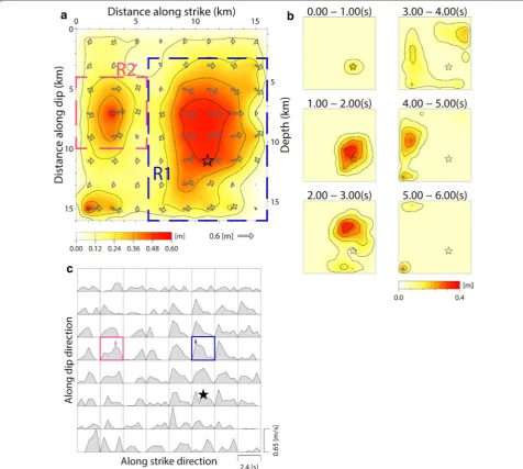
Figure 2a shows the total slip distribution on the fault. The seismic moment is 2.1 × 10¹⁸ Nm (Mw 6.1). Vftw is set to 3.3 km/s, which provides the smallest-misfit solu-tion among all solusolu-tions for Vftw varying from 1.6 to 4.0 km/s. A large-slip region, with a maximum slip of 0.6 m, extends from the rupture staring point to the shallower part (R1 in Fig. 2a). Another large-slip region, with a maximum slip of 0.5 m, is located to the NNW of
(See figure on previous page.)
the rupture starting point (R2 in Fig. 2a). The area and the slip values of R1 are larger than those of R2; hence, the released seismic moment on R1 is approximately five times larger than that on R2. Figure 2b, c shows the snapshots of the rupture progression and the slip-veloc-ity time function on each subfault. After the rupture initiation, the rupture mainly propagated from the rup-ture staring point in the upward direction, and contin-ued for 3 s, causing large slips on R1. Then, the rupture
propagated in the NNW direction at 3–5 s, causing large slips on R2. The total rupture duration is approximately 5 s.
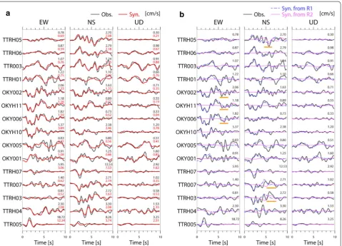
Figure 3a shows the comparison between the observed and synthetic waveforms. The waveform fit is satisfac-tory. Figure 3b shows the contribution of the two large regions, R1 and R2 in Fig. 2a, to the synthetic waveforms. At all stations, the contribution of R1 is large. The contri-bution of R2 is small compared to that of R1. However, Fig. 2 a Total slip distribution on the fault. The slip contour interval is 0.12 m. Vectors denote the direction and the amount of the slip on the hang-ing wall side. Open star denotes the rupture starthang-ing point. Rectangles with blue and magenta broken lines indicate the regions with large slips defined in this study, R1 and R2, respectively. b Rupture progression in terms of slip amount for each 1.0 s interval. The slip contour interval is 0.08 m.
Page 5 of 10 Kubo et al. Earth, Planets and Space (2017) 69:127
seismic waveforms radiating from R2 are necessary to explain the later part of the observed waveforms at sev-eral stations with different azimuths such as TTR007 and OKY006, highlighted with orange bars in Fig. 3b. This result suggests that the slips in R2 are not an artifact.
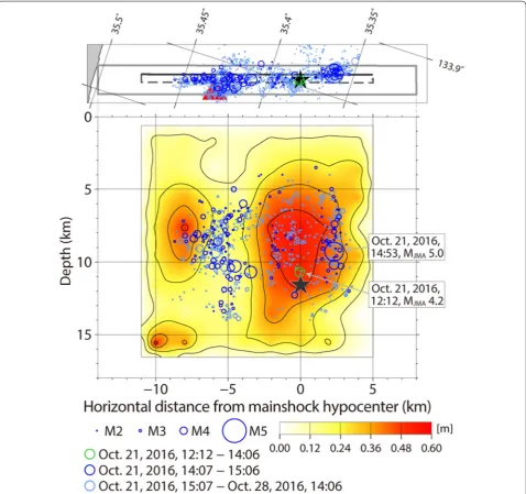
Figure 4 shows the comparison between the slip distri-bution and the spatial distridistri-bution of aftershocks. Many aftershocks occurred around the areas with large slips (>0.4 m) for 1 h after the mainshock, whereas only a few aftershocks occurred within the areas. The aftershocks mainly occurred in the area located approximately 2 km SSE of the mainshock hypocenter (south part of R1) and in the area located approximately 4–7 km NNW of the main-shock hypocenter (north part of R1 and south part of R2). The largest aftershock (October 21, 2016, 14:53 JST, MJMA 5.0) occurred on the south part of R1. In addition, the area of high seismicity within 1 week after the mainshock did not overlap with the large coseismic slip area, although some aftershocks with relatively small magnitude (M < 3) occurred on R1. The feature that aftershocks are not active
where coseismic slips are large in the mainshock has also been found in other crustal strike-fault-type earthquakes in Japan: the 1995 south Hyogo (Kobe) earthquake (MJMA 7.2) (e.g., Hirata et al. 1996; Ide et al. 1996), the 2000 west-ern Tottori earthquake (e.g., Ohmi et al. 2002; Semmane et al. 2005), the 2005 west off Fukuoka earthquake (MJMA 7.0) (e.g., Nishimura et al. 2006; Uehira et al. 2006), and the first large event (MJMA 6.5, April 14, 2016, JST) of the 2016 Kumamoto earthquakes (e.g., Asano and Iwata 2016; Kubo et al. 2016). In the largest event (MJMA 7.3, April 16, 2016, JST) of the 2016 Kumamoto earthquakes, some aftershocks occurred in the area with large coseismic slips along the Futagawa fault, while the number of the after-shocks was relatively small compared to other regions such as the Hinagu fault and the Aso area (e.g., Asano and Iwata 2016; Kubo et al. 2016). Figure 4 also shows the spa-tial distribution of foreshocks approximately 2 h prior to the mainshock. The foreshocks, including the largest one (October 21, 2016, 12:12 JST, MJMA 4.2), occurred near the hypocenter of the mainshock.
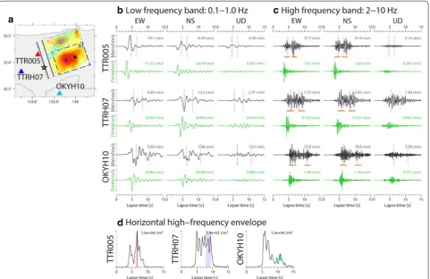
Next, we focus on the relationship between the source rupture process of the 2016 central Tottori earthquake and ground motions observed at near-fault stations. Velocity waveforms at three near-fault stations, TTR005 (K-NET Kurayoshi), TTRH07 (KiK-net Sekigane), and OKYH10 (KiK-net Kamisaibara) (Fig. 5a), in the low fre-quency band (0.1–1.0 Hz) are plotted in Fig. 5b. This fre-quency band is equal to that in the source inversion. The low-frequency waveforms at the near-fault stations have a large pulse at horizontal components. The large pulse
is mostly formed by the contribution of R1, and the low-frequency waveforms from R2 have small amplitudes compared to those from R1 (Fig. 3b). The large amplitude of the low-frequency waveforms from R1 is primarily caused by the large seismic moment release on R1. The difference in the total rupture duration on R1 and R2 could also affect the amplitude difference of the low-fre-quency waveforms from them; the long rupture duration on R1 could cause a lower dominant frequency of wave-forms from R1 than that of wavewave-forms from R2.
Page 7 of 10 Kubo et al. Earth, Planets and Space (2017) 69:127
Figure 5c shows velocity waveforms at the near-fault stations during the 2016 central Tottori earthquake in the high frequency band (2.0–10 Hz). The high-frequency horizontal waveforms at these stations have two major wave packets, highlighted with orange bars. Figure 5b, c also shows velocity waveforms during the largest fore-shock that occurred near the mainfore-shock hypocenter (Figs. 4, 5a) and had a left-lateral strike-fault-type mecha-nism similar to the mainshock (Fig. 1b). Compared to the mainshock waveforms, the foreshock waveforms are sim-ple: one wave packet in the high frequency band and one pulse in the low frequency band. The arrival time of the first wave packet in the mainshock waveforms is similar to that of the wave packet in the foreshock waveforms.
suggests that the radiation region of the second wave packet is located to the north of the radiation region of the first wave packet. The potential radiation region of the second wave packet is estimated using the arrival times of the second wave packet in horizontal high-frequency envelope at TTR005 and OKYH10 (Fig. 5d). The details of the analysis are provided in the Additional file 1. The estimated radiation region of the second wave packet (cyan shade in Fig. 5a) is located on the north side of the fault and overlaps R2 in our source model, suggest-ing that the second wave packet might radiate from R2. We calculate theoretical arrival times of direct S-waves radiating from the center of the largest-slip subfaults in R1 and R2 at the peak time of their slip velocities (Fig. 2c) and plot them in Fig. 5c (blue and magenta lines). Their theoretical arrival times roughly correspond to the observed two wave packets at the near-fault stations and can explain the observed variation in the arrival-time dif-ferences among the stations. Thus, it is likely that the two wave packets observed at the near-fault stations corre-spond to the two significant ruptures at R1 and R2 in our source model. However, these discussions are qualitative and further studies are required to directly estimate the spatiotemporal pattern on radiation strength of high-fre-quency waveforms.
The waveform appearance in the high frequency band at the near-fault stations differs from that in the low fre-quency band (Fig. 5): while the low-frequency waveforms have a small amplitude at the time corresponding to the second wave packet, the second wave packet in the high frequency band has a large amplitude compared to the first wave packet. Although the amplitude ratio between the first and second wave packets in the high frequency waveforms differs among stations, the amplitude differ-ence is smaller in the high frequency band than that in the low frequency band. The large amplitude of the sec-ond wave packet in high-frequency waveforms is likely due to the dominant frequency of the waveforms from R2 being higher than that of the waveforms from R1 because of the compact fault rupture of R2. In addition, the radiation pattern of body waves, which largely affects the spatial amplitude pattern in the low frequency band, is distorted at frequencies over 1 Hz mainly due to the seismic wave scattering and diffraction within the hetero-geneous crust (e.g., Liu and Helmberger 1985; Takemura et al. 2016). Both of these factors lead to the reduction in the amplitude difference shown in the low frequency band; however, they are not enough to explain the larger amplitude of the second wave packet than the first one in the high-frequency waveforms at TTR005. A likely rea-son is the combination of the non-geometric attenuation with frequency dependence and the short distance from R2. In general, high-frequency waveforms over 1 Hz are
likely to be largely affected by the intrinsic and scattering attenuations compared to the low-frequency waveforms. Because the distance from R2 to TTR005 is shorter than that from R1, the amplitude of the high-frequency wave-forms radiating from R2 was less affected by the intrinsic and scattering attenuations, causing the large amplitude of the second wave packet in the high-frequency wave-forms at TTR005.
Conclusions
In this study, we investigated the source process of the 2016 central Tottori earthquake using a multiple-time-window kinematic waveform inversion. We used the strong motion waveforms (0.1–1.0 Hz) at 15 stations. In the estimated source model, the seismic moment and the maximum slip are 2.1 × 10¹⁸ Nm (M
w 6.1) and 0.6 m, respectively. The source model has two large-slip regions: a region with the maximum slip that extends from the hypocenter to the shallower part (R1), and another with smaller slips located to the NNW of the hypocenter (R2). The released seismic moment on R1 is five times larger than that on R2. Many aftershocks occurred around areas with large coseismic slips, whereas only a few aftershocks occurred within the areas, as observed in other crustal strike-fault type earthquakes in Japan. This earthquake had the foreshock activity near the mainshock hypo-center approximately 2 h before the mainshock.
The contribution of R1 to seismic waves in the low frequency band (0.1–1.0 Hz), which is the analysis fre-quency band of the waveform inversion, is significant at all stations. Although the contribution of R2 is smaller than that of R1, the seismic waveforms radiating from R2 are necessary to explain the later part of the observed waveforms at several stations with different azimuths. At near-fault stations, two major wave packets were observed in the high frequency band (2.0–10 Hz), and the variation in their arrival times among the near-fault stations indicates that the two wave packets are likely to correspond to the fault ruptures on R1 and R2. The wave-form difference in high- and low-frequency bands at the stations can be qualitatively explained using our source model.
Abbreviations
JMA: Japan Meteorological Agency; NIED: National Research Institute for Earth Science and Disaster Resilience; NNW: north-northwest; PGA: peak ground acceleration; SSE: south-southeast.
Additional file
Page 9 of 10 Kubo et al. Earth, Planets and Space (2017) 69:127
Author details
1 National Research, Institute for Earth Science and Disaster Resilience, 3-1, Tennodai, Tsukuba, Ibaraki 305-0006, Japan. 2 Disaster Prevention Research Institute, Kyoto University, Gokasho, Uji, Kyoto 611-0011, Japan.
Authors’ contributions
HK analyzed the data, interpreted the results, and drafted the manuscript. WS, SA, and HS participated in the design of the study and the interpretation of the results. All authors read and approved the final manuscript.
Acknowledgements
We thank Prof. K. Asano, the editor, and two anonymous reviewers for their helpful comments. We used the unified hypocenter catalog provided by JMA and the 10-m mesh DEM published by the Geospatial Information Authority of Japan. We used Generic Mapping Tools (Wessel and Smith 1998) to draw the figures.
Competing interests
The authors declare that they have no competing interests.
Publisher’s Note
Springer Nature remains neutral with regard to jurisdictional claims in pub-lished maps and institutional affiliations.
Received: 13 April 2017 Accepted: 4 September 2017
References
AIST (National Institute of Advanced Industrial Science and Technology) (2007) Active fault database of Japan, December 13, 2007 version. AIST, Tsukuba Akaike H (1980) Likelihood and the Bayes procedure. In: Bernardo JM, De
Groot MH, Lindley DV, Smith AFM (eds) Bayesian statistics. University Press, Valencia, pp 143–166
Aoi S, Kunugi T, Nakamura H, Fujiwara H (2011) Deployment of new strong motion seismographs of K-NET and KiK-net. In: Earthquake Data in Engineering Seismology. Geotechnical, Geological and Earthquake Engineering, vol 14. Springer, Dordrecht, pp 167–186. doi:10.1007/978-94-007-0152-6_12
Asano K, Iwata T (2016) Source rupture processes of the foreshock and main-shock in the 2016 Kumamoto earthquake sequence estimated from the kinematic waveform inversion of strong motion data. Earth Planet Space 68:147. doi:10.1186/s40623-016-0519-9
Bouchon M (1981) A simple method to calculate Green’s function for elastic layered media. Bull Seismol Soc Am 71(4):959–971
FDMA (Fire and Disaster Management Agency) (2017) The 2016 central Tottori earthquake (35th report). http://www.fdma.go.jp/bn/2016/detail/977. html. Accessed 21 Aug 2017 (in Japanese)
Fujiwara H, Kawai S, Aoi S, Morikawa N, Senna S, Kudo N, Ooi M, Hao KX, Hayakawa Y, Toyama N, Matsuyama H, Iwamoto K, Suzuki H, Liu Y (2009) A study on subsurface structure model for deep sedimentary layers of Japan for strong-motion evaluation. Techical Note 337, National Research Institute for Earth Science and Disaster Prevention, Tsukuba, Japan (in Japanese)
Fukuyama E, Ishida M, Dreger DS, Kawai H (1998) Automated seismic moment tensor determination by using on-line broadband seismic waveforms. J Seism Soc Jpn (Zisin 2) 51:149–156 (in Japanese with English abstract)
Fukuyama E, Ellsworth WL, Waldhauser F, Kubo A (2003) Detailed fault structure of the 2000 Western Tottori, Japan, earthquake sequence. Bull Seismol Soc Am 93:1468–1478
Hartzell SH, Heaton TH (1983) Inversion of strong ground motion and tel-eseismic waveform data for the fault rupture history of the 1979 Imperial Valley, California, earthquake. Bull Seismol Soc Am 73(6):1553–1583
Hirata N, Ohmi S, Sakai S, Katsumata K, Matsumoto S, Takanami T, Yamamoto A, Iidaka T, Urabe T, Sekine M, Ooida T, Yamazaki F, Katao H, Umeda Y, Naka-mura M, Seto N, Matsushima T, Shimizu H, Japanese University Group of the Urgent Joint Observation for the 1995 Hyogo-ken Nanbu Earthquake (1996) Urgent joint observation of aftershocks of the 1995 Hyogo-ken Nanbu earthquake. J Phys Earth 44(4):317–328
Ide S, Takeo M, Yoshida Y (1996) Source process of the 1995 Kobe earthquake: determination of spatio-temporal slip distribution by Bayesian modeling. Bull Seismol Soc Am 86(3):547–566
Iida M (1990) Optimum strong-motion array geometry for source inversion—II. Earthq Eng Struct Dyn 19:35–44
Iida M, Miyatake T, Sshimazaki K (1988) Optimum strong-motion array geom-etry for source inversion. Earthq Eng Struct Dyn 16:1213–1225 Iwata T, Sekiguchi H (2002) Source process and near-source ground motion
during the 2000 Tottori-ken Seibu earthquake. Paper presented at 11th Japan Earthquake Engineering Symposium. The Japanese Geotechnical Society, Tokyo (in Japanese with English abstract)
Kanamori H (1972) Determination of effective tectonic stress associated with earthquake faulting, the Tottori earthquake of 1943. Phys Earth Planet Inter 5:426–434
Kaneda H, Okada A (2002) Surface rupture associated with the 1943 Tottori earthquake compilation of previous reports and its tectonic geomorpho-logical implications. Act Fault Res 21:73–91 (in Japanese with English abstract)
Kennett BLN, Kerry NJ (1979) Seismic waves in a stratified half space. Geophys J R Astr Soc 57:557–583
Kubo H, Suzuki W, Aoi S, Sekiguchi H (2016) Source rupture processes of the 2016 Kumamoto, Japan, earthquakes estimated from strong-motion waveforms. Earth Planet Space 68:161. doi:10.1186/s40623-016-0536-8
Lawson CL, Hanson RJ (1974) Solving least squares problems. Prentice-Hall, Old Tappan
Liu H, Helmberger DV (1985) The 23:19 aftershock of the 15 October 1979 Imperial Valley earthquake: more evidence for an asperity. Bull Seismol Soc Am 75(3):689–708
Nishida R (1990) Characteristics of the 1983 Tottori earthquake sequence and its relation to the tectonic stress field. Tectonophys 174(3–4):257–278 Nishimura T, Fujiwara S, Murakami M, Suito H, Tobita M, Yarai H (2006) Fault model of the 2005 Fukuoka-ken Seiho-oki earthquake estimated from coseismic deformation observed by GPS and InSAR. Earth Planet Space 58(1):51–56. doi:10.1186/BF03351913
Ohmi S, Watanabe K, Shibutani T, Hirano N, Nakao S (2002) The 2000 Western Tottori Earthquake—seismic activity revealed by the regional seismic networks. Earth Planet Space 54(8):819–830. doi:10.1186/BF03352075
Olson AH, Apsel RJ (1982) Finite faults and inverse theory with applica-tions to the 1979 Imperial Valley earthquake. Bull Seismol Soc Am 72(6A):1969–2001
Saito M (1978) An automatic design algorithm for band selective recursive digital filters. Geophys. Explor. (Butsuri-Tanko) 31:112–135 (in Japanese with an English abstract)
Sekiguchi H, Irikura K, Iwata T (2000) Fault geometry at the rupture termina-tion of the 1995 Hyogo-ken Nanbu earthquake. Bull Seismol Soc Am 90(1):117–133
Semmane F, Cotton F, Campillo M (2005) The 2000 Tottori earthquake: a shal-low earthquake with no surface rupture and slip properties controlled by depth. J Geophys Res 110:B03306. doi:10.1029/2004JB003194
Suzuki W, Aoi S, Sekiguchi H (2010) Rupture process of the 2008 Iwate–Miyagi Nairiku, Japan, Earthquake derived from near-source strong-motion records. Bull Seismol Soc Am 100(1):256–266. doi:10.1785/0120090043
Takemura S, Kobayashi M, Yoshimoto K (2016) Prediction of maximum P- and S-wave amplitude distributions incorporating frequency- and distance-dependent characteristics of the observed apparent radiation patterns. Earth Planet Space 68:166. doi:10.1186/s40623-016-0544-8
Usami T, Ishii H, Imamura T, Takemura M, Matsuura R (2013) Materials for com-prehensive list of destructive earthquakes in Japan, 599–2012. University of Tokyo Press, Tokyo (in Japanese)
Wald DJ, Helmberger DV, Heaton TH (1991) Rupture model of the 1989 Loma Prieta earthquake from the inversion of strong-motion and broadband teleseismic data. Bull Seismol Soc Am 81(5):1540–1572
Wessel P, Smith WHF (1998) New, improved version of Generic Mapping Tools released. EOS Trans Am Geophys Union 79:579