An algorithm for deriving core magnetic field models from the Swarm data set
Martin Rother, Vincent Lesur, and Reyko Schachtschneider
Helmholtz Centre Potsdam, GFZ German Research Centre for Geosciences, Telegrafenberg, 14473, Germany
(Received March 1, 2013; Revised June 28, 2013; Accepted July 17, 2013; Online published November 22, 2013)
In view of an optimal exploitation of the Swarm data set, we have prepared and tested software dedicated to the determination of accurate core magnetic field models and of the Euler angles between the magnetic sensors and the satellite reference frame. The dedicated core field model estimation is derived directly from the GFZ Reference Internal Magnetic Model (GRIMM) inversion and modeling family. The data selection techniques and the model parameterizations are similar to what were used for the derivation of the second (Lesuret al., 2010) and third versions of GRIMM, although the usage of observatory data is not planned in the framework of the application to Swarm. The regularization technique applied during the inversion process smoothes the magnetic field model in time. The algorithm to estimate the Euler angles is also derived from the CHAMP studies. The inversion scheme includes Euler angle determination with a quaternion representation for describing the rotations. It has been built to handle possible weak time variations of these angles. The modeling approach and software have been initially validated on a simple, noise-free, synthetic data set and on CHAMP vector magnetic field measurements. We present results of test runs applied to the synthetic Swarm test data set.
Key words: Satellite, Earth observation, magnetism, main field, SHA model, Swarm.
1.
Introduction
The pioneering satellite Magsat (Langelet al., 1982), the Danish satellite Oersted and the low earth orbiting satel-lite CHAMP have opened opportunities for the investiga-tion of the various contribuinvestiga-tions to the Earth’s magnetic field (e.g. the main field, the lithospheric field, the external fields), but also of their interactions and impacts on our so-ciety. In the light of recent perception from palaeomagnetic records, indicating surprisingly fast magnetic field reversals (Nowaczyket al., 2012), and in view of the fast evolution of the field revealed by CHAMP satellite data (Lesuret al., 2008), it is important to pursue data collection, which is foundation for global studies of core dynamics and core-mantle interaction. The Swarm mission with three satel-lites, two flying side by side and one in a higher orbit, and its well-suited instrumentation, is able to contribute to this objective. A backbone for magnetic field investigations is to have a valid, consolidated, ideally up-to-date magnetic field model describing the main field contribution originat-ing in the Earth’s fluid core. The focus implies a reliable description of its time derivatives: the elusive small scale Secular Variation (SV) and Acceleration. Depending on the interest of the modelers and the time period in focus, several approaches with different model designs are avail-able, e.g. CM4 (Sabakaet al., 2004), POMME (Mauset al., 2006), CHAOS (Olsenet al., 2010) and GRIMM (Lesur et al., 2008, 2010) series.
To help with the successful exploitation of the expected
Copyright cThe Society of Geomagnetism and Earth, Planetary and Space Sci-ences (SGEPSS); The Seismological Society of Japan; The Volcanological Society of Japan; The Geodetic Society of Japan; The Japanese Society for Planetary Sci-ences; TERRAPUB.
doi:10.5047/eps.2013.07.005
Swarm data, ESA has supported a processing environment to create so-called Level 2 products (Olsenet al., 2013). The aim is to provide the scientific community with state-of-the-art models of the known different contributions to the magnetic field. The products are grouped into two cate-gories: The CAT-2 products, with mature and strongly au-tomatized algorithms creating Level 2 products with small delays, and, the CAT-1 software based on mature and ac-cepted algorithms that require scientific supervision. De-scribed in the following is the outline of the so called Dedi-cated Core field Model (DCO) branch of the Swarm CAT-1 processing environment.
The DCO software is split into a slow and a fast lane. Each lane is split in the determination of the dedicated core field model and an estimation of the misalignment angles between magnetic field sensors and the satellite reference frame. The slow lane is designed to cover all available data and therefore is suited for time-spans of at least one year. The fast lane focuses on short periods but requires nonethe-less to cover all local times, i.e. generally about at least three or four months. While the slow lane aims at a precise de-scription of the secular variation, and is therefore character-ized by a complex description of the time dependencies, the main goal of the fast lane is to have an early view on the accuracy of the predictive core field model used by other Swarm CAT-1 chains. Also the fast lane is used to assess the validity of the misalignment angles between magnetic field sensors and the satellite reference frame used for the processing of the Swarm Level-1b magnetic data (Tøffner-Clausen and Hansen, 2007). The outputs of the fast lane are for internal validation only and not released to the public. They are not described any further in this manuscript.
The structure of the paper is as follows: the DCO core
field modeling and the misalignment angle (i.e. Euler angle) estimations are introduced in separate sections, even though they are an integral part of the software. For each of these we first present an outline of the algorithm, and then the specific adaptation for the Swarm set-up. Finally the DCO processing approach is tested and applied to a synthetic data set established in the framework of this study. Results of application to real data are also shown for the Euler Angle determination.
2.
Core Field Modeling: Heritage and
Adapta-tions
The GRIMM approach was established and developed with the rapidly growing CHAMP data set and the char-acteristics of the model have been generally preserved in this implementation. Nonetheless, a few changes have been introduced in the focus of the approach and in its applica-tion. It is not foreseen to use observatory data. However, it is mainly in the handling of the external and induced fields that the approach has evolved. A careful selection of their parametrization is necessary, firstly since the mod-eling needs to be based on the available indices, secondly since other indices than in the usual GRIMM approach are used, and thirdly because of the specific characteristics of the data set actually at hand. As modelling the core field from satellite data is a difficult process, a Scientist in Loop (SIL) is required to adjust the software configuration and make final decisions for delivery.
2.1 Selection
The first step in the modeling attempt is to decimate and select the available data to remove data carrying signals that cannot be separated from the core field signal, or that cannot be modeled in detail, or finally that are generally noisy. Local time windows, various indices and flags are used as selection criteria. The important distinction is between the polar region with magnetic latitudes outside the±55◦range on one hand and the mid- and low-latitude satellite data on the other. For the latter, data are rotated to the Solar Magnetic (SM) system of coordinates. The following series of indices related to the external field are used as input for the selection criteria:
MMA is the a time series of spherical harmonic model coefficients of the large-scale magnetospheric field and its Earth-induced counterparts (Hamilton, 2013); AUX DST is the name of a Swarm L2 Product with DST
indices including quick-look and preliminary esti-mates from World Data Center for Geomagnetism in Kyoto, in listing format (Olsenet al., 2013);
AUX IMF is the name of a Swarm L2 Product with the values of the Interplanetary Magnetic Field propagated to the Earth magnetosphere (Olsenet al., 2013).
The following selection criteria apply:
- the z-component of the interplanetary magnetic field (IMF-Bz) must be positive, for minimizing the noise
associated with possible re-connection of the mag-netic field lines with the Interplanetary Magmag-netic Field (IMF);
- a 20 s minimum is required between sampled points for minimizing correlated errors generated by
non-modeled lithospheric field;
- data local time must be between 23:00 and 05:00 for min-imizing the contribution from the magnetic field gener-ated in the ionosphere. The sun must also be below the horizon at 100 km above the Earth’s reference radius (a =6371.2 km),
- the value of theMMAmust be less than 30 nT and its time derivative norm lower than 100 nT/day to select mag-netically quiet periods. While the original GRIMM scheme is using the Vector Magnetic Disturbance In-dex, Thomson and Lesur (2007), with bounds set to 20 nT and 100 nT/day, our selection is using either the fast MMA product or, the AUX DST product. The choice is made depending on the availability of the MMA or whether or not the MMA turns out to be not appropriate for the purpose. The thresholds used will need adapting to the actual data set. It is one of the tasks of the SIL to choose and justify the choice. - the quality flags should indicate data of a minimum
qual-ity threshold. This is set mainly to reject outliers. Data with only one star camera reading should normally be rejected unless the weak data density requires their se-lection. The handling of the flag information has been implemented as for CHAMP data, but cannot actu-ally be fine-tuned for Swarm before true readings from Swarm are available.
Outside the±55◦ magnetic latitude interval, at high lati-tudes, the three component vector magnetic satellite data are used in North, East, Center (NEC) system of coordi-nates and for all local times. These two selection criteria were chosen to avoid significant gaps in the time series of high-latitude data. Even if these selection criteria are used for the initial core field inversion, they may be tuned by the SIL if this seems recommended by the initial results. In par-ticular, for the application to the synthetic Swarm test data set (TDS-1, see Olsen et al., 2013) the high latitude data were selected with a tight time window.
2.2 Model parametrization and estimation
The current section describes the model parametrization based mainly on the GRIMM inversion scheme. The al-gorithm does not attempt to estimate either the magnetic toroidal fields generated by the field-aligned currents, or the field generated in the ionosphere at high latitudes. As it has been found from a comparison between GRIMM and a preliminary version of GRIMM-2, modeling these fields improves the fit to the data only marginally. Apart from the lithospheric field, the model includes the core field, a rep-resentation of the large scale external fields and their asso-ciated internally induced counterparts. The core fieldBcis modeled as the gradient of an internal potential field given as a series of spherical harmonics (SHs) (Lesuret al., 2008):
wherec = 3485 km is the Earth’s core reference radius, Ym
l (θ, φ) are the Schmidt semi-normalized SHs.
Nega-tive orders, m < 0, are associated with sin(|m|φ)terms, whereas null or positive orders,m ≥0, are associated with cos(mφ)terms. The maximum SH degree Lcfor the core field model is set toLc=20, even if the contribution of the lithospheric field is known to be significant at these SH de-grees. The time dependency of the Gauss coefficientsgml (t)
is represented as a series ofNtB-splines,ψi6(t), of order 6.
The knots are chosen to be half a year apart. This spline or-der, increased during the development of the GRIMM inver-sion family since the first verinver-sion, focuses on the estimation of the secular variation and acceleration. The spline knot spacing of half a year is taken from the third generation of the GRIMM model family.
The field generated in the lithosphere is assumed to be independent of time and defined by:
Bl= −∇Vl(θ, φ,r) (4)
wherea = 6371.2 km is the Earth’s reference radius and Llthe maximum degree for the lithosphere. As in the sec-ond and third versions of GRIMM, a reference lithospheric field model is subtracted from the data in the pre-processing phase. Because of that, the present modeling effort ef-fectively corresponds to a correction of the original litho-spheric field model. The maximum SH degree for this cor-rection is not required to be large and is generally set be-tween 20 and 30. In the specific application to the TDS-1 the SH maximum degree was set to 20, this means no litho-spheric field coefficients were determined and the reference lithospheric field model is the AUX-LIT field model (Olsen et al., 2013), used in DCO usually truncated to max SH de-gree 60. This model is a single-epoch snapshot represented as spherical harmonic expansion with coefficients from or-der 16 to 250 and will remain unchanged at least during the first few years of the Swarm mission.
The handling of the large scale external fields in principle distinguishes between firstly, a magnetospheric field model in the solar magnetic system of coordinates (SM) varying slowly in time and, secondly, a fast varying external field model, combined with its induced counterpart. This lat-ter field is in the usual earth fixed, earth cenlat-tered system of coordinates (geocentric), and parametrized in time by an index controlling the rapid variations of the field. The exter-nal field index is preferentially the MMA Level 2 product (Hamilton, 2013). In case the MMA index is not available or found not to be appropriate, the DST index can be used alternatively.
Assuming, the MMA index is used, the external field for the slowly varying part is described by
Be= −∇(e(θ, φ,r,t)) , (6)
where it is understood that the vectors and coordinates are in SM system. The temporal variations of the external Gauss coefficientsqm
l (t)are defined by a piecewise constant
repre-sentation with a 100 day knot spacing. This knot definition is consistent with a preprocessing of the MMA data that in-cludes removing 100 day averages over the full time series. For the fast varying part the external field is described by:
Bm= −∇(m(θ, φ,r,t)), (9)
The external and internal part of the MMA series,mmae
j(t)
andmmaij(t)control the time dependencies and are scaled
on 100 day periods byq˜l jm,g˜ m
l j, respectively.
The maximum SH degree for the external field is set to Le = 2, but only a certain subset of the external coeffi-cients may actually be used depending on the data set and the apparent significance of the coefficients. Particularly for the test using the TDS-1 data set, only the orders 0 and±1 were chosen for the slowly varying external field model, whereas for the fast varying fields parametrized with the MMA index only the SH degree 1 and the order 0 SH de-gree 2 coefficients were included. Later application on real measurements may require an adaptation of these settings. 2.3 Procedures
Calculating a core magnetic field model consists of esti-mating the Gauss coefficients defining the model such as to minimize the functional:
where thewiare weights, thediare magnetic data readings
at(θi, φi,ri,ti)in the directionηi, andBci,Bli,Bei,Bmi
are vector model values at the same positions. TheFi(gml )
are functions of the core field Gauss coefficients that can be used to constrain the core field model behaviour. In a matrix form this reduces to:
=(d−Gm)tW(d−Gm)+mtD m, (14)
where the model vectormis made of the Gauss coefficients of the models, the matrixGcan be derived from the expres-sions of the model given in the previous section (Eqs. (1)– (12)) and d is the data vector. Normally, the problem is linear and in principle can be solved rapidly, but the defini-tion of the weight matrixWand the data selection process require an iterative process to be set up.
ex-ternal field description. For this first step we assume a Gaus-sian distribution of the residuals. The mid-latitude dipole-aligned Z-component data are used exclusively for the ex-ternal field part and do not enter into the estimation of the core field. This is equivalent to the infinite variance ap-proach set in Olsenet al.(2007) and therefore requires sev-eral iterations of the optimization process until further up-dates in the model parameters become insignificant. The model nonetheless requires some constraints to be set on the temporal evolution of the core field model. These con-straints are introduced through the matrix D in the func-tional defined in Eq. (14). We use effectively the same ap-proach as in the second and third version of GRIMM de-scribed in Lesuret al.(2010), where the acceleration is min-imized at the end points of the model whereas the third time derivative is minimized over the model time span. But it is not excluded that we revise this approach if necessary.
At this stage the distributions of the data residuals for all components and data types are inspected in order to estimate the parameterskandαof slightly modified Huber-Weights (Olsen, 2002). These weights are defined by:
w(x)=
1 if|x| ≤k
k
|x|
2−α
if|x|>k . (15)
Recommended values forkare approximately 1, and setting
α = 1 gives exactly Huber-Weights. For residual values in between±k, a Gaussian distribution is assumed. These weights require an iterative re-weighted least squares ap-proach (Farquharson and Oldenburg, 1998) and the iterative process is stopped when changes in the model parameters become insignificant.
3.
Euler Angles
The main instruments for estimating the orientation of the magnetic sensors in space are the star cameras. These are rigidly mounted on the so-called “optic bench” that also carries the magnetometers. So, in principle, the angles (i.e. Euler angles) between the magnetic sensors and the star cameras are known and should not vary in time. However, since the satellites are under stress during the launch and sustain large temperature gradients along their orbit path, it is known that these angles have to be re-estimated during the flight. The algorithm we shortly describe below for this purpose is fundamentally the same as the one proposed in Olsen et al. (2007), but we use quaternions here. Small corrections to the Euler angles established before launch can be estimated, assuming a known magnetic field and using the magnetometer readings to find their orientations. Alternatively, we can co-estimate the magnetic field model and the Euler angles. This latter algorithm is described below after an introduction to quaternions.
3.1 Quaternions
Rotations, in particular those describing the attitude of the magnetic sensors relative to the satellite reference frame can be given in quaternion format. The quaternions were in-vented by Sir William Rowan Hamilton in 1843 and form a four-dimensional normalized division algebra over the real numbers—i.e. a quaternion is defined by four real values, usually noted (q1,q2,q3,q4). They allow for a
continu-ous, pole-free representation of rotations. They also allow for a numerically proper nesting and interpolation of tions (they are typically used to efficiently describe rota-tions, as in computer graphics). The quaternions are nor-malized such that:
1=q12+q22+q32+q42 (16)
The representation of a rotation matrix is then (from Wertz, 1978):
R= ⎡ ⎣q
2
1−q22−q32+q42 2(q1q2+q3q4) 2(q1q3−q2q4)
2(q1q2−q3q4) −q12+q22−q32+q42 2(q2q3+q1q4)
2(q1q3+q2q4) 2(q2q3−q1q4) −q12−q22+q32+q24 ⎤ ⎦. (17)
In the following, the notation of the quaternion is us-ing the convention proposed in Wertz (1978), p. 762, equa-tion E-7a. Here,q4 is the scalar component of the rotation whereas(q1,q2,q3)defines the rotation axis. We note that a given rotation is described by a unique quaternion as long as the sign ofq4is imposed.
3.2 Algorithm
Finding the Gauss coefficients describing the measured magnetic field reduces, as described in the previous section, to solving a linear system:
d−G m=0, (18)
where constraints applied to the core field model are ig-nored for simplicity. The extension to that case is straight-forward, as these constraints do not enter the algorithm de-veloped for the Euler angle estimation.
We can rewrite this equation for an iterative scheme at iterationkas:
δdk=d−G mk
=Gδm (19)
withmk+1 =mk+δm. The data vectordis expressed in
an Earth-fixed system of coordinates. It is calculated from the readings in the sensor system of coordinatesdsthrough
two successive rotations:
d=R(t)R ds, (20)
whereRis the rotation from the sensor system to the satel-lite reference frame that we want to estimate, andR(t)is a rotation that is given and depends on the measured satellite position and orientation. The relation betweenRand the quaternion is given in Eq. (17) and the linear system (18) can be written:
R(t)R ds−G m=0. (21)
Since the matrixRhas a non-linear dependence relative to the quaternion, this system is solved iteratively. At iteration kit can be written:
δdk=dk−G mk
=Gδm−i4=1δqi R∂∂Rqikds, (22)
where the data vectordkhas an indexkbecause it depends
As for the magnetic model parameters we have: qi,k+1 = qi,k+δqi. The matrices ∂∂Rqik are easily calculated from the
Eq. (17).
Unfortunately, finding the model parameters and the quaternions by solving the linear system of Eq. (22) it-eratively through least squares does not impose that the Eq. (16) is maintained. It may be imposed by explicit re-normalization after each iteration before updating the dk,
but it is much more efficient to implement the constraint di-rectly in the inversion scheme. The quaternions are updated byqi,k+1=qi,k+δqi and we have to impose:
1=
i
qi2,k+1. (23)
After neglecting the second order terms this leads to:
1−
i
qi2,k =2
i
qi,kδqi (24)
The set of Eqs. (22) and the Eq. (24) must be solved si-multaneously for theδmand [δqi]{i=1:4}, the latter equation
should be scaled by a large factor for the constraint to be fully efficient.
3.3 Procedures
We have organized the software to cover two operation modes that consist of either estimating the core field model and the quaternions independently, or of co-estimating both. The need to cover these two operation modes changed the internal data organization in comparison to the original GRIMM scheme. With the introduction of the quaternions and rotation matrices, the problem becomes clearly non-linear and more than one iteration is required. The estima-tion of the core field model independently also requires sev-eral iterations. The software is therefore organized with two embedded iterative loops, the outer loop being used to han-dle the non-linearity of the quaternion determination. The data are therefore read in the sensor system of coordinates and the outer loop includes, as an initial task, a rotation of these data in an Earth-fixed system using the current val-ues of the quaternions. It is always possible to reduce the complexity of the problem by either imposing a core field model, in which case the inner loop is skipped, or by im-posing a set of quaternions with the possibility of reading directly the data in an Earth-fixed system of coordinates. In all cases, it is the iterative re-weighted least-squares algo-rithm used in GRIMM model family that is applied to solve the system of equations.
As there is a possibility that the Euler angles vary with time, for example as a result of a thermal bending of the optical bench, the quaternions have to be parametrized in time. Our approach is to split long time spans into relatively short segments where the quaternions are assumed constant. The objective is to have segments covering no more than 30 days, while a full local time coverage, achieved typically in 4 months for one satellite, is still necessary to derive robust core field models. This 30 day window requirement imposes a different data selection scheme is applied for the quaternion estimation than for the core field estimation. For stability of the quaternion estimation it is essential to select a significant number of vector data for each segment. This is typically achieved by selecting data on a larger local time
window than the tight 23:00 to 05:00 window used for core field modeling.
The stability of the quaternion estimation is expected to be a critical issue, so we apply the following scheme. A first estimation is done on a relatively large window (e.g. 100 days) that is progressively reduced to 30 days. This pro-vides good starting values for the non-linear estimation and the new quaternions determined on smaller time window can be required not to differ too much from the starting val-ues. Outliers, destabilizing the quaternion estimation, can be also hand-picked and removed from the data set. A clear advantage of the scheme is that it gives us hints about the overall robustness of the estimates.
The distinct 30 days segments for the Euler angle deter-mination may become very unequally populated. To avoid invalid results, low population thresholds apply, and the re-sulting gaps in the Euler Angle time series may be filled by interpolation. Ultimately the most robust segment may rep-resent the final quaternion estimate if a fairly smooth tem-poral variation of the angles is assumed.
4.
Tests
The basic functionality of the software has been fully tested on an ideal synthetic vector data set, where the noise and external fields were ignored and an ideal distribution of data on the sphere was assumed. The performances of the algorithm were extensively tested on the data sets defined below. Results are given in the next section.
4.1 Data sets
Tests were conducted on two data sets:
• The full CHAMP data set covering 10 years from 2001 to 2010;
• TDS-1, a synthetic multicomponent data set used for closed loop and processing tests. External, internal and induced fields as well as noise were taken into account for generating this data set, but the field contributions associated with the field aligned currents were not in-cluded. This TDS-1 was supplied by DTU (see Olsen et al., 2013) and the Swarm Science Study (Olsen et al., 2007). The data are provided in two systems of coordinates: In a North-East-Center (NEC) system and in the sensor system of coordinates. In the latter a time constant misalignment error was introduced for each satellite, in order to test the Euler angle estima-tion process.
5.
Results
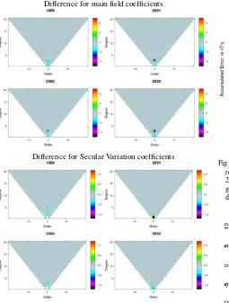
Difference for main field coefficients
Difference for Secular Variation coefficients
Fig. 1. Comparison of the estimated DCO coefficients with the given reference core field model coefficients. The unscaled differences for the main field are shown in upper part of figure, the unscaled differences for the secular variations are shown in its lower part. These differences are presented for four snapshots inside the data span.
Table 1. Standard deviations of the residuals to the fit to the data in nT.
Satellite ABC A B C
Type
X (SM) 2.76 2.73 2.72 2.84
Y (SM) 2.93 2.87 2.87 3.06
X (HL) 7.51 7.67 7.67 7.16
Y (HL) 6.05 6.18 6.21 5.72
Z (HL) 6.23 6.35 6.38 5.91
The final fit to the selected data extracted from the TDS-1, gives residuals with standard deviations usually about 2– 3 nT for the mid- and low latitude regions, and 6–7 nT for the polar area (see Table 1). We note that standard devia-tions for the polar residuals are smaller than the values ob-tained with CHAMP data (Lesuret al., 2010). At mid- and low-latitudes, the values are similar to those obtained with GRIMM-2, but significantly larger than those obtained with GRIMM-3. Again this is probably due to the specificity of the data set rather than to the modeling and parametrization approach.
The absolute differences between the obtained core field model and the reference model Gauss coefficients are shown for four selected epochs in the upper part of Fig. 1. Corresponding results for the SV are also shown in the
Fig. 2. The figure shows the contribution for each order to the overall requirement function in nT/year as a function of time over days since 2000.0. The 3 nT/y requirement limit is marked as horizontal dashed gray line. The increasing deviation towards the begin and end of the data covered period are obvious.
Fig. 3. Differences from known misalignment angles as a function of time for each 30 day window after removal of outliers and underpopulated segments. Data gaps are interpolated. Theγ angle, in particular on satellite C (highest orbit) shows largest differences. The horizontal dashed lines at 3 arcsecs are the Swarm threshold requirement standard deviation.
lower part of this figure. The absolute difference of g3 0 is anomalously large, but this difficulty has never been ob-served when handling real data. The absolute differences for the SV are small.
To assess the quality of the SV model, an errorE(l)has been defined by:
E(l,t)=
(l+1)+l
m=−l
g˙m
l (t)− ˙grml (t)
2
(25)
where g˙m
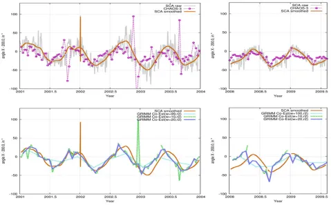
Fig. 4. The first component of the XYZ (or equivalentlyα, β, γ) Euler rotation angles calculated for CHAMP data for 2001 to 2004 (left part) and late period 2008 and 2009 (right part). Upper frames: Estimates from other modelers, see text. Lower frames: GRIMM/DCO results for various constant Euler angles segment length.
core field Gauss coefficients andg˙rml their reference values.
Figure 2 shows this error for each SH degreel, for 2≤l ≤ 16, as a function of time. The deviation, that is generally small, increases at the beginning and end of the data time span. The value for the threshold requirement for Swarm, 3 nT/y, is indicated by the horizontal dashed gray line.
For determining the misalignment angles, we follow the scheme presented in the previous section. We determine a good (constant) starting value of the misalignment an-gles by initially using a large segmentation window. After subsequently reducing the Euler angle segmentation win-dow size, the result for a 30-day winwin-dow length is shown in Fig. 3. The misalignment angles introduced in the TDS-1 are different for each satellite, but constant in time. Devi-ations from a constant value in Fig. 3 is evidence of noisy estimates. A removal of outliers and underpopulated seg-ments has already been done and gaps in the time series are interpolated linearly. The result of this interpolation step is particularly obvious for theαangle (green), satellite-B, starting at MJD 0. The value for the threshold requirement for Swarm, a standard deviation of 3 arcsecs, is indicated by the horizontal dashed gray lines. The scatter is largest for the gamma angle (rotation around the Z direction), par-ticularly for satellite C (satellite C has the highest orbit alti-tude).
6.
Discussion
The core field modeling works well under the condi-tions of the given Swarm test data set, the fit to the data is good. As stated above, from our experience with the
CHAMP data, the standard deviations of the residuals in polar regions are significantly too small compared to what we expect from real data. This is probably because no field-aligned current models are used when generating the syn-thetic data set. However, for equatorial regions, the resid-uals’ standard deviations are slightly larger than expected, possibly associated with unexpected contributions from ei-ther the ionosphere or the induced magnetic field models.
The benefit of using quaternions for the Euler angle deter-mination is the simplicity of the algorithm for their deriva-tion. But, as a drawback, the quaternion norm needs to be constrained, which for DCO is imposed through regulariza-tion. The Euler angle estimation on TDS-1 is leading to results within the ESA threshold requirements for the Eu-ler angle estimation on Swarm. The γ angles are clearly the most noisy; this is to be expected from the near-polar configuration of the orbits. The same difficulty has been observed with real satellite data.
estima-tions from Stefan Maus, the so-called SCA series), and from Nils Olsen, the so called CHAOS-3 series, see Olsenet al. (2009). Both Euler angles time series were provided by per-sonal communication. The presented tests for the Euler an-gle estimation on CHAMP data had been performed about the end of the active mission of CHAMP using the stage of the processing at that time and using the corresponding Eu-ler angle time series from the external modeEu-lers available at that time. The CHAMP data had been reprocessed mean-while a couple of times and fully corrected public CHAMP magnetic field data may not show all features revealed on that earlier stage.
In the lower frame of Fig. 4 the GRIMM versions dif-fer by the estimation window length in days (w =99, 10, 20); ther2in the label indicates an additional data ing applied to CHAMP data to reduce outliers. This filter-ing was removfilter-ing data vectors with current data residuals after inversion larger then constant thresholds, which can be set in the configuration for each component and data type. The thresholds chosen are intended to remove ap-parent short periods of outlier bursts, probably created by suboptimal external field handling. In particular the shown Euler angle X reveals a possibly spurious strong local time dependency, which is common to all estimates. Deviations can result from compromises on complexity (i.e. in external field modeling), from the size of the local time window and from the size of the Euler angle temporal segments. The sensitivity of the DCO-based Euler angle determination to model details appears weak, but the sensitivity to sparse-ness of segment population and data quality is strong. This is particularly true when a model-angle co-estimation ap-proach is used. As shown on the upper frame of Fig. 4, for the rotation along the X component, the rotations we obtain are generally in agreement with the available refer-ences: the apparent local time dependence, also present in the SCA reference series, is mostly reproduced.
The amplitude of the angleα local time dependence is about 30–50 arc secs. This is large in comparison to the requirement of only a few arc secs for the Euler angle esti-mation performance for Swarm. However, the mechanism behind those strong local time dependences of the angle is not finally clarified, even though it is generally agreed that the dependence is likely to be a signature of the field gener-ated by field aligned currents. This hypothesis is supported by the results obtained with the TDS-1 where, beside the scattering, no spurious signal in the time series of the Euler angle correction estimations is visible (see Fig. 3). The field aligned currents are one prominent external field contribu-tion, that is not properly simulated in the TDS-1. On the other hand, even though the local time dependency is not correlating consistently with the measured temperature sig-nal (private communication with Hermann L¨uhr), a bending of the optical bench cannot be excluded. It will be interest-ing to see, if actual Swarm measurements of vector data lead to any significant local time dependent modulation of the Euler angle time series, as has been experienced with CHAMP. Also remarkable is the existence of a remain-ing local time signal in the difference between the GRIMM Euler angle series and the smoothed SCA solution. This difference looks like a phase shift starting from 2002.5 or
shortly after. The appearance of this time-shift is yet unex-plained. For short time windows (e.g. 10 days) the angles estimation for the CHAMP data starts to be noisy. For ex-ample the scatter of the results is significant in the SCA estimation, for which we also show a version where a sym-metric smoothing filter has been applied (see Fig. 4). For our approach, a good compromise between roughness and resolution is found for a window of 20 days (w=20). The optimum results obtained here for the window of 20 days may be attributed to the fact that this choice minimizes the effects of magnetosphere related to magnetic storm activity. The duration of a typical magnetic storm is shorter then this 20 day period.
Finally, we note that the results for the other two rotation angles (not shown) do not present clear patterns. The Z rotation (i.e. theγangle) is always the most noisy estimate.
7.
Conclusion
Two distinct approaches are integrated in the dedicated core field modeling for Swarm, estimating a core field and estimating the Euler angles. The algorithms have been ex-tensively tested using the Swarm TDS-1. The results show that we are able to recover the reference Gauss coefficients used to build the synthetic data set with a very good accu-racy. However, the quality of the core field modeling results when applied to real data can only be assessed if the data se-lection parameters, the external field model parametrization and the constraints applied to the model are tuned by the “scientist in the loop”. We are confident that the approach we follow can be successful because it has been used on CHAMP satellite data. The estimation of the Euler angles has also been fully tested, on CHAMP data, where the re-sults resembled prominent features revealed by other mod-elers. Nonetheless, we will have to wait for probably a full year of Swarm data before being able to assess the separa-tion of the external field from the angles estimates.
Acknowledgments. We thank the anonymous reviewers for the helpful comments. We thank other members of the SCARF con-sortium for constructive discussions and ESA for financial sup-port. We thank Stefan Maus and Nils Olsen for providing time series of Euler Angle estimates. The figures have been created ei-ther with the free statistic software R (R Development Core Team, 2012), or Gnuplot.
References
Farquharson, C. G. and D. W. Oldenburg, Non-linear inversion using gen-eral measures of data misfit and model structure,Geophys. J. Int.,134, 213–227, 1998.
Hamilton, B., Rapid modelling of the large-scale magnetospheric field from Swarm satellite data,Earth Planets Space,65, this issue, 1295– 1308, 2013.
Langel, R., R. Estes, and G. Mead, Some new methods in geomagnetic field modeling applied to the 1960-1980 epoch,J. Geomag. Geoelectr., 34, 327–349, 1982.
Lesur, V., I. Wardinski, M. Rother, and M. Mandea, GRIMM: the GFZ Reference Internal Magnetic Model based on vector satellite and ob-servatory data, Geophys. J. Int., 173, 382–394, doi:10.1111/j.1365-246X.2008.03724.x, 2008.
Lesur, V., I. Wardinski, M. Hamoudi, and M. Rother, The second genera-tion of the GFZ Reference Internal Magnetic field Model: GRIMM-2,
doi:10.1029/2006GC001269, 2006.
Nowaczyk, N. R., H. W. Arz, U. Frank, J. Kind, and B. Plessen, Dynamics of the Laschamp geomagnetic excursion from Black Sea sediments,
Earth Planet. Sci. Lett., 351, 54–69, doi:10.1016/j.epsl.2012.06.050, 2012.
Olsen, N., A model of the geomagnetic main field and its secular variation for epoch 2000 estimates from Ørsted data,Geophys. J. Int.,149, 454– 462, 2002.
Olsen, N., T. J. Sabaka, and L. R. Gaya-Pique, Study of an Improved Comprehensive Magnetic Field Inversion Analysis for Swarm, Final Report, Tech. Rep. ESA CONTRACT No 11570/05/NL/AR, Danish National Space Center (DNSC), 2007.
Olsen, N., M. Mandea, T. J. Sabaka, and L. Tøffner-Clausen, CHAOS-2—a geomagnetic field model derived from one decade of continuous satellite data,Geophys. J. Int.,179, 1477–1487, doi:10.1111/j.1365-246X.2009.04386.x, 2009.
Olsen, N., M. Mandea, T. Sabaka, and L. Tøffner-Clausen, The CHAOS-3 geomagnetic field model and candidates for the 11th generation IGRF,
Earth Planets Space,62, 719–727, doi:10.5047/eps.2010.07.003, 2010. Olsen, N., E. Friis-Christensen, R. Floberghagen, P. Alken, C. D Beggan, A. Chulliat, E. Doornbos, J. T. da Encarnac¸˜ao, B. Hamilton, G. Hulot, J. van den IJssel, A. Kuvshinov, V. Lesur, H. L¨uhr, S. Macmillan, S. Maus, M. Noja, P. E. H. Olsen, J. Park, G. Plank, C. P¨uthe, J. Rauberg, P. Rit-ter, M. Rother, T. J. Sabaka, R. Schachtschneider, O. Sirol, C. Stolle,
E. Th´ebault, A. W. P. Thomson, L. Tøffner-Clausen, J. Vel´ımsk´y, P. Vi-gneron, and P. N. Visser, TheSwarmSatellite Constellation Application and Research Facility (SCARF) andSwarmdata products,Earth Plan-ets Space,65, this issue, 1189–1200, 2013.
R Development Core Team: R: A Language and Environment for Statisti-cal Computing, R Foundation for StatistiStatisti-cal Computing, Vienna, Aus-tria, http://www.R-project.org, 2012.
Sabaka, T. J., N. Olsen, and M. E. Purucker, Extending compre-hensive models of the Earth’s magnetic field with Ørsted and CHAMP data,Geophys. J. Int., 159, 521–547, doi:10.1111/j.1365-246X.2004.02421.x, 2004.
Thomson, A. W. P. and V. Lesur, An improved geomagnetic data selection algorithm for global geomagnetic field modelling,Geophys. J. Int.,169, 951–963, doi:10.1111/j.1365-246X.2007.03354.x, 2007.
Tøffner-Clausen, L. and F. Hansen, Swarm Phase B, Level 1b Proces-sor Algorithms, Tech. Rep. SW-RS-DSC-SY-0002, Issue 3, Danish Na-tional Space Center (DNSC), 2007.
Wertz, J. R. ed.,Spacecraft Attitude Determination and Control, vol. 73 of
Astrophysics and Space Science Library, Kluwer Academic Publishers, 1978.