Deriving the geomagnetically induced electric field at the Earth’s surface
from the time derivative of the vertical magnetic field
Heikki Vanham¨aki1, Ari Viljanen1, Risto Pirjola1,2, and Olaf Amm1
1Finnish Meteorological Institute, P.O. Box 503, FI-00101 Helsinki, Finland
2Natural Resources Canada, Geomagnetic Laboratory, 7 Observatory Crescent, Ottawa, Ontario, K1A 0Y3, Canada (Received November 4, 2011; Revised November 15, 2012; Accepted March 22, 2013; Online published October 9, 2013)
We present a new method for estimating the geomagnetically induced electric field at the Earth’s surface directly from the time derivative of the vertical magnetic field, without any need for additional information about the Earth’s electric conductivity. This is a simplification compared to the presently used calculation methods, which require both the magnetic variation field and ground conductivity model as input data. The surface electric field is needed e.g. in modeling Geomagnetically Induced Currents (GIC) that flow in man-made conductor systems, such as gas and oil pipelines or high-voltage power grids. We solve the induced electric field directly from Faraday’s law, by representing the magnetic variation field in terms of external equivalent current and taking time derivative of the associated vector potential. This gives an approximative solution, where the divergence-free part of the electric field is reproduced accurately (at least in principle), but the curl-divergence-free part related to lateral variations in ground conductivity is completely neglected. We test the new calculation method with several realistic models of typical ionospheric current systems, as well as actual data from the Baltic Electromagnetic Array Research (BEAR) network. We conclude that the principle of calculating the (divergence-free part of the) surface electric field from time derivative of the vertical magnetic field is sound, and the method works reasonably well also in practice. However, practical applications may be rather limited as the method seems to require data from a quite dense and spatially extended magnetometer network.
Key words:Geoelectric field, geomagnetically induced current, GIC, space weather.
1.
Introduction
Temporal variations in ionospheric current systems cre-ate an electric field in the Earth that is further modified by the induced telluric current flowing in the conducting ground. Knowledge of the resulting induced electric field at the Earth’s surface is needed e.g. in modeling Geomag-netically Induced Currents (GIC) that flow in man-made conductor systems, such as gas and oil pipelines or high-voltage power grids (e.g. Pirjola, 2002). GIC modeling is usually done in two steps: 1) Calculate the horizontal elec-tric field at the Earth’s surface and 2) calculate the current driven by the electric field in a specific conductor system. In this article we concentrate on the first step, where the ap-propriate horizontal length scale is of the order of 100 km, corresponding to the typical segment length of power grids or pipelines (e.g. Viljanenet al., 2004).
Direct measurements of the ground electric field are not commonly available at suitable spatial scales, as they are sensitive to local conductivity structures (e.g. Jiracek, 1990; Groom and Bahr, 1992), so for GIC purposes the induced electric field is usually calculated from magnetic measure-ments. Several methods have been developed for this task (e.g. Pirjola, 2002; Pulkkinenet al., 2003a; Viljanenet al.,
Copyright cThe Society of Geomagnetism and Earth, Planetary and Space Sci-ences (SGEPSS); The Seismological Society of Japan; The Volcanological Society of Japan; The Geodetic Society of Japan; The Japanese Society for Planetary Sci-ences; TERRAPUB.
doi:10.5047/eps.2013.03.013
2004; McKay and Whaler, 2006; Thomson et al., 2009 and references therein), but they require some knowledge of the Earth’s electric conductivity as input (typically 1D conductivity model or the regional impedance tensor that connects horizontal magnetic and electric disturbances). In this article we discuss the possibility of calculating the in-duced electric field more directly, using Faraday’s law and measured time derivative of the vertical component of the ground magnetic field.
Direct integration of Faraday’s law has previously been used e.g. by Vanham¨akiet al.(2007) and Vanham¨aki (2011) in ionospheric induction studies. However, as far as we know, this method has not been employed in GIC studies. In magnetotellurics (MT) the vertical magnetic field is com-monly utilized in the form of tipper vectors, that connect the horizontal and vertical magnetic disturbances (e.g. Gough, 1989; Zhanget al., 1993; Egbert, 2002; Jozwiak, 2011 and references therein). In principle, knowledge of the tipper vector and impedance tensor on a sufficiently dense and spatially extended grid allows one to form a complete and self-consistent description of the electromagnetic fields at the ground surface, without knowing the detailed 3D con-ductivity structure (Beckenet al., 2008).
However, in MT the primary goal is to investigate the conductivity structure of the ground, whereas in GIC stud-ies the surface electric field itself is the main result of the geophysical investigation (step 1 above). Thus the full machinery developed in MT, e.g. division of the observed
field into normal and anomalous parts, is not necessarily needed in GIC studies. Furthermore, much of the MT the-ory is based on assuming quasi-uniform external sources in the ionosphere (e.g. see discussion by Chave and Wei-delt, 2012), although some source effects may be included (e.g. Egbert, 2002). In high-latitude GIC studies this ap-proximation is usually not valid, as large GIC events can be produced by relatively small scale ionospheric current sys-tems (e.g. Viljanenet al., 2001; Pulkkinen et al., 2003c), and even the substorm electrojets may not be considered quasi-uniform if the analysis area (e.g. power grid) is large. However, it should be noted that in GIC studies it is usually enough to include source effects when interpolating the ob-served magnetic field, but the surface electric field can then be calculated using local plane wave approximation at each location separately (e.g. Viljanenet al., 2004).
In this study our goal is to develop as simple and straight-forward way of calculating the surface electric field as pos-sible. The calculation method should preferably work in the space/time domain and use only directly measurable data as input, without any knowledge of the Earth’s conductivity structure or any assumptions about the ionospheric currents.
2.
Theory
We consider only the horizontal part of the induced elec-tric field at the Earth’s surface, i.e. a 2D vector field on a sphere. According to Helmholtz’s theorem we can always represent it as a sum of curl-free (cf) and divergence-free (df) parts,
and subscripthdenotes the horizontal components. In Sub-sections 2.1 and 2.2 we will show that the divergence-free electric field is purely inductive and can be calculated from Faraday’s law, while the curl-free part is associated with charge accumulation caused by horizontal conductivity gra-dients in the ground.
It should be noted that the decomposition into curl- and divergence-free parts is unique only if it’s done globally. In regional studies where the analysis area is some hundreds or thousand km across, there may be an additional “Laplacian” part that has zero curl and zero divergence inside the anal-ysis area. In this study we will neglect the Laplacian part, which may cause some errors in regional studies. However, the errors are expected to diminish as the analysis area in-creases.
The above division into curl- and divergence-free parts can be compared with the common practice in magnetotel-lurics, where the electromagnetic surface field is divided into tangential-electric (TE) and tangential-magnetic (TM) modes (e.g. Beckenet al., 2008; Chave and Weidelt, 2012). In the TE (TM) mode the electric (magnetic) field has no vertical component at the ground surface. In the general case with 3D ground conductivity variations the TE and TM modes are coupled to each other, but in 2D cases they can be separated into E-polarization and B-polarization modes by choosing the coordinate system appropriately. With 1D ground conductivity structure (layered in vertical direction)
the TE and TM modes degenerate to the same poloidal-magnetic mode. This is often assumed as the normal mode in MT studies, so that the anomalous fields are created by additional 2D or 3D conductivity structures.
The 1D normal mode is purely inductive, and so is the whole TE mode in a 2D situation. In contrast, the anoma-lous part of the 2D TM mode (i.e. deviation from the normal mode) is caused by charge accumulation at the conductivity gradient. In the general 3D situation the TE and TM modes are mixed, but it is still reasonable to assume that TE mode is mostly inductive while the anomalous part of TM mode is heavily affected by charge accumulation (Beckenet al., 2008). Thus we see thatEdfh in Eq. (1) can be identified with
the TE mode (here including the normal mode), whileEcf
h
is associated with the anomalous part of the TM mode. 2.1 Divergence-free electric field
We can solve the divergence-free part of the electric field directly from Faraday’s law,
using the measured vertical magnetic disturbanceBr as the
input data. We can represent the divergence-free electric field in terms of a potential, asEdfh = −ˆer × ∇ψ, so that
Eq. (3) forms a Poisson’s equation forψ. However, there are two issues in solving Eq. (3) this way. We must interpo-late the vertical magnetic field inside the (sometimes rather sparse) magnetometer network in a physically sensible way and unless we have global data coverage we have to specify some boundary conditions forψ.
Becken and Pedersen (2003) and Becken et al. (2008) show how the TE mode impedance tensor and electric field can be calculated from measured tipper vectors, without knowing the 3D ground conductivity structure. In their method the hypothetical normal magnetic disturbance is given, and the anomalous TE mode magnetic field is solved iteratively. Then the anomalous TE mode surface electric field can be calculated by solving Faraday’s law in Eq. (3) in frequency/wavenumber domain. The total TE electric field, equal to the divergence-free fieldEdfh, is obtained by
adding the normal part from a separate (distant) measure-ment. While this approach seems to work well, and might be useful for hypothetical event analysis of GIC characteris-tics, we want to develop a more straightforward space/time domain algorithm, where previously measured tipper vec-tors are not required.
One convenient way to solve Eq. (3) in space/time do-main is the Spherical Elementary Current Systems (SECS) method introduced by Amm (1997) and Amm and Viljanen (1999). In the SECS method the magnetic disturbance field is represented in terms of an equivalent current that is com-posed as a sum of elementary systems. It has been shown to be a very flexible and robust method for determining iono-spheric equivalent currents (Amm and Viljanen, 1999; Wey-gandet al., 2011), separating the ground magnetic varia-tion field into internal and external parts (Pulkkinenet al., 2003b) and interpolating the surface magnetic field (Pulkki-nenet al., 2003a; McLay and Beggan, 2010).
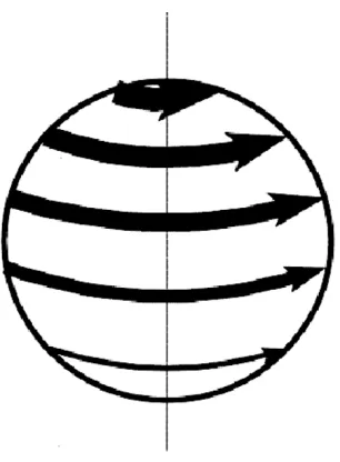
Fig. 1. Divergence-free Spherical Elementary Current System (SECS). From Amm and Viljanen (1999).
magnetic field below the ionosphere as the real external (ionospheric + magnetospheric) currents. According to the potential theory such a solution always exists and is uniquely defined in global scale (see discussion in Haines and Torta, 1994; Amm and Viljanen, 1999). However, the measured magnetic disturbance also has internal (induced) sources, in addition to the external currents. This means that we cannot represent all 3 components of the disturbance field usingJeq,extalone. Rather, we can represent either the vertical or the horizontal part withJeq,ext. In previous GIC studies emphasis has often been on the horizontal magnetic field (e.g. Viljanenet al., 2001; Pulkkinenet al., 2003a and references therein), but in this study the vertical magnetic field is needed in Faraday’s law.
We note that in principle we could model the whole mea-sured magnetic disturbance field, both vertical and horizon-tal parts at the same time, by adding another layer of in-ternal equivalent current to model the inin-ternal sources, as done e.g. by Pulkkinenet al.(2003b). We tested this two-layer approach with the numerical examples described in Section 3, but concluded that it does not significantly im-prove the solution for the surface electric field. Explana-tion is that according to potential theory the vertical part of the magnetic disturbance field can be represented solely by
Jeq,ext, even if part of the disturbance is caused by internal sources (see discussions by Haines and Torta, 1994; Amm and Viljanen, 1999). AdditionalJeq,int are needed only if both vertical and horizontal disturbances are modeled at the same time.
The divergence-free SECS functions defined by Amm (1997) and illustrated in Fig. 1 form a set of basis func-tions for representing any (continuously differentiable) divergence-free vector field on a sphere. The external equivalent current is determined so that elementary sys-tems are placed in a suitable grid at a higher altitude and their magnitudes are chosen so that the resulting magnetic field fits the observations as closely as possible (e.g. in the least squares sense). Usually the equivalent current layer is
placed at∼100 km, just below the real ionospheric currents, but smaller heights can be used to interpolate the magnetic measurements at dense magnetometer networks. In this study we use 100 km height in order to filter out smaller scale structures that are not really needed at GIC studies, although it means that agreement with local surface electric field measurements (see Subsection 3.3) may get slightly worse. More details about grid selection and the fitting pro-cess are given e.g. by Amm and Viljanen (1999), Pulkkinen
et al.(2003b) and Weygandet al.(2011).
For each individual time-step we collect the vertical com-ponents of the measured ground magnetic disturbance at lo-cationsrn=(RE, θn, φn)into one vector
while the unknown scaling factors of the elementary sys-tems located atrelk =(RI, θkel, φkel)are collected into another
the external (ionospheric) equivalent current layer. These vectors are connected by a transfer matrixT, so that
BB B BBB B
Br =T·IIIIIIIIsecs. (6)
Elements of the transfer matrixTgive the vertical magnetic field caused by each individual unit SECS at the magne-tometer sites, and is therefore known and depends only on geometry. For example, Tn,k gives the vertical magnetic
field atrn caused by the SECS centered atrelk. Details how
to calculate the matrixTare given in Appendix A, while Amm and Viljanen (1999) and Weygandet al.(2011) dis-cuss how to invert Eq. (6) for the unknown scaling factors
IIIIIIIIsecsusing truncated singular value decomposition. The inversion of Eq. (6) is done for each time-step sepa-rately, but using the same elementary system grid (locations
relk). This means that the matrixT has to be inverted just
once for each magnetometer network. In this study our ele-mentary system grid is located between 56◦–73◦North and
−8◦–52◦ East, with 0.6◦ resolution in latitude and 1.4◦ in longitude, so that it extends few degrees outside the conti-nental BEAR and IMAGE magnetometer networks shown in Fig. 2. The optimum truncation point in SVD for the IM-AGE, BEAR and “Ideal” networks used in Section 3 was chosen to minimize the least-squares error in the resulting electric field. Thus 13 out of 18, 16 out of 36 and 154 out of 825 singular values were used in analyzing the data from IMAGE, BEAR and “Ideal” networks, respectively.
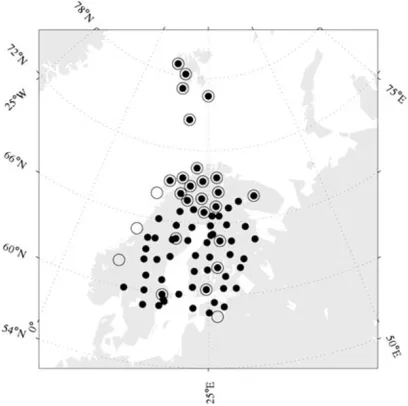
Fig. 2. The permanent IMAGE magnetometer stations (open circles) and the temporary stations (solid black) that formed the BEAR network in June–July 1998. Only the continental stations below 72◦North are used in this study.
contains the horizontal components of the vector potential andS is another transfer matrix that is described in Ap-pendix B. According to the definition of the vector poten-tialB = ∇ ×Aand in the Coulomb gauge used by Amm and Viljanen (1999)∇h·Ah = 0, so we can calculate the
divergence-free part of the surface electric field from Eq. (3) simply as
Edfh = −
∂Ah
∂t . (9)
2.2 Curl-free electric field
The curl-free part of the surface electric field is more dif-ficult to calculate. As discussed above and in Beckenet al.
(2008), it is equal to the anomalous part of TM mode elec-tric field, and vanishes if there are no horizontal gradients in ground conductivity (1D layered ground).
If the conductivity σ (RE, θ, φ) of the ground surface
layer is known, we can write the surface current as
jh(RE, θ, φ)=σ
Edfh +Ecfh. (10)
The total current is divergence-free, so divergence of the surface current can be written as
∇σ·Edfh + ∇ ·
σEcfh
= −∂(jr)
∂r , (11)
where−jr is the vertical current flowing downwards from
the surface. If we could assume that vertical currents near the ground surface are vanishingly small, we could solve the curl-free part of the surface electric field from Eq. (11), as-suming that the surface conductivity is known. Another op-tion is to use the anomalous part of the TM mode impedance tensor, which can be deduced from the total and TE mode impedance tensors as shown by Beckenet al.(2008). How-ever, if the total impedance tensor were known in the whole analysis area with good enough spatial resolution, then the surface electric field could be calculated directly from the
measured (and interpolated) magnetic field, without any need to solve Eqs. (3) and (11). This is rarely the situation in GIC studies, although McKay and Whaler (2006) have used this approach in a rather small spatial area.
Equation (11) shows how divergence ofEcfh is associated
with sharp conductivity gradients, such as coast lines (e.g. Jiracek, 1990; Gilbert, 2005), where the term∇σ ·Edfh is
large. However, the electric field Ecfh itself may extend
hundreds or even thousand km outside these regions (e.g. Fergusonet al., 1990).
In the present study we will simply assume that curl-free part of the electric field is zero,
Ecfh =0. (12)
This is equivalent to ignoring the TM mode. The main rea-son for this assumption is that our primary goal in this study is to find a simple way to estimate the surface electric field directly from magnetic data, without any knowledge of the ground conductivity. An attempt to solveEcfh from Eq. (11)
would violate this principle. However, we also note that in present GIC studies it is common practice to use calcula-tion methods where the curl-free electric field is ignored, e.g. plane wave method combined with 1D ground conduc-tivity structure (Viljanen et al., 2004), and these seem to give useful results. This indicates that in many (or even most) situations the divergence-free electric field is much more important than the curl-free field, at least in the spa-tial scales involved in GIC modeling.
However, it should be kept in mind that our assumption in Eq. (12) is a reasonable approximation at best, and in some situations, where charge accumulation due to large conduc-tivity gradients dominates the surface electric field, it may be completely unrealistic. Thus our calculation method de-scribed in Subsection 2.1 produces only the divergence-free part of the electric field, equivalent to the sum of the TE-mode and non-anomalous part of the TM-TE-mode. This ap-proximation may well explain why some of our results with BEAR data (discussed in Subsection 3.3) were less than op-timal.
3.
Test Examples
We can test the calculation method presented in the pre-vious section by constructing realistic test cases where the correct surface electric field is known. We also present one test case using magnetic and electric measurements from the Baltic Electromagnetic Array Research (BEAR) net-work, which operated for about 1.5 months during June– July 1998 (Korjaet al., 1998).
3.1 Electrojet
Our first test case is a simplified oscillating electrojet, which we model by placing a line current at an altitude
H above the Earth’s surface. According to Boteleret al.
(2000) this is equivalent to a sheet current at a lower altitude with a Cauchy-type current distribution. Ground induction is modeled by placing a perfect conductor at depthhbelow the surface. We place the electrojet at latitude 65◦, directly above the IMAGE and BEAR networks illustrated Fig. 2.
Fig. 3. Profiles of the surface electric and magnetic fields along longitude 23◦East (see Fig. 2) for a simple 1D electrojet model. Top panel shows the vertical magnetic field, middle panel the horizontal (North component) magnetic field and bottom panel the horizontal (East component) electric field. The model distribution is plotted with solid line, and the results calculated using IMAGE and BEAR stations (see Fig. 2) with dash-dotted and dashed lines, respectively.
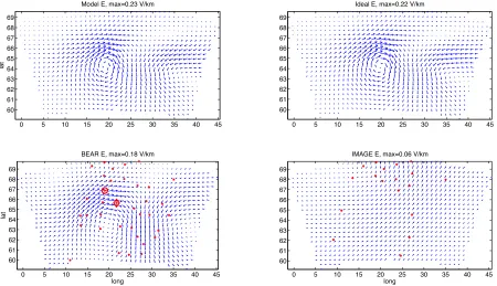
Fig. 4. The model surface electric field (top left) for the WTS system, together with the results calculated using an ideal magnetometer network (top right), BEAR network (bottom left) and IMAGE network (bottom right). Locations of the BEAR and IMAGE stations are indicated by asterisks in the corresponding plots. Additionally, the BEAR stations Jokkmokk and Boden used in Subsection 3.3 are marked with a circle and diamond, respectively.
projection for the station coordinates. For an East-West ori-ented line current the surface fields are simply (Boteleret al., 2000)
B=μ0I
2π
Heˆx−xeˆz H2+x2 +
(H+2h)eˆx+xeˆz
(H+2h)2+x2
, (13)
E=−μ0
2π
d I dt ln
(H+2h)2+x2
√
H2+x2
ˆ
ey. (14)
wherez = 0 is the ground surface and the line current is centered at x = 0. In our example we use values H =
2π/300 s−1. These fields are evaluated at the IMAGE and BEAR stations and the radial magnetic field is used as input in the SECS-based calculation method, without correcting for the difference between local Cartesian and spherical geometry. The IMAGE and BEAR networks are relatively small (we neglect stations above 72◦North, see Fig. 2), so this simplification does not cause significant errors.
The correct North-South profiles of the surface electric and magnetic fields as well as the results calculated using ∂tBr from the IMAGE and BEAR stations are illustrated in
Fig. 3, which shows a cut along 23◦meridian. From the up-per panel we see that the vertical part (z-component) of the magnetic field is very well reproduced from the BEAR ob-servations, and even the sparser IMAGE array gives a rea-sonable estimate. In contrast, the middle panel shows that the horizontal part (in this case x-component) is coarsely underestimated. This is a direct consequence of the calcu-lation process where only the vertical field is used as the input, as the ground induced currents tend to decrease the vertical magnetic field but increase the horizontal field. Re-sults for the horizontal surface electric field (in this case
y-component) are illustrated in the bottom panel. Taking into account the small distortions caused by the simpli-fied geometry, we conclude that the electric field calculated from the BEAR network is in very good agreement with the model and even the more sparse IMAGE array gives rea-sonable results for the 1D electrojet.
3.2 Data-based model
A more concrete test can be performed by using realistic, data-based models of typical ionospheric current systems. Here we use model of a westward traveling surge (WTS) constructed by Amm (1995). Ground induction is modeled using the Complex Image Method (CIM, Wait and Spies, 1969; Thomson and Weaver, 1975; Boteler and Pirjola, 1998; Pirjola and Viljanen, 1998). The CIM calculation gives the electric and magnetic fields at the Earth’s surface as a sum of external and internal parts, once the temporal evolution of the primary external (ionospheric) current sys-tem and 1D Earth conductivity structure are specified. In this study we use a layered ground model that is suitable for Central Finland (see figure 4 by Viljanen and Pirjola, 1994) and create time evolution of the WTS system by moving the static model westward at a constant speed of 10 km/s. More discussion about the WTS model as well as the CIM calculation process are given by Vanham¨akiat al.(2005), who used the same approach to study the feedback effect of ground induction on the ionospheric current system.
Figure 4 shows the surface electric field calculated for the WTS model using the CIM procedure (top left panel), as well as the electric fields estimated fromBrusing simulated
measurement at different magnetometer networks. The re-sult labeled as “Ideal” makes use of Br at every available
point of the CIM modeling area, which is a 1100 km (lat-itude)×1800 km (longitude) grid with 50 km spacing in both horizontal directions. The result from this Ideal net-work is in excellent agreement with the original model. Also the result based on the simulated measurements at the BEAR stations (bottom left panel) captures the overall structure of the surface electric field and also the magnitude is reasonably accurate. The main error in the BEAR result
seems to be underestimation of the electric field magnitude and spreading of small-scale features into too large areas.
On the other hand, the result based on the IMAGE net-work is practically useless. This may be caused by the fact that according to Fig. 4 the scale size of the WTS system is smaller than the typical magnetometer separation of the IMAGE array. However, the moderate deterioration of our results when changing from the Ideal network to the dense BEAR, compared to the large drop in quality when chang-ing to the more sparse IMAGE may also indicate some in-trinsic limitation of the calculation method with respect to spatial resolution of the input data.
It should be noted that in the previous electrojet ex-ample and in this WTS test the surface electric field is purely rotational. The curl-free part of the surface electric field is exactly zero, as there are no horizontal gradients in ground conductivity. Thus our calculation method may have given too promising results, as in reality our assump-tion in Eq. (12) is never exactly satisfied.
3.3 BEAR data
Our final test utilizes direct measurements of the surface electric and magnetic fields collected with the BEAR net-work. The largest event during BEAR operation, a sub-storm with maximum local AE index of∼1300 nT, took place in the morning hours of 26 June 1998. The surface electric field recorded at most of the BEAR stations was usually severely modified by local conductivity anomalies, but there are a few stations where the measuredEh should
give a good estimate of the large scale surface electric field around the station (T. Korja, private communication).
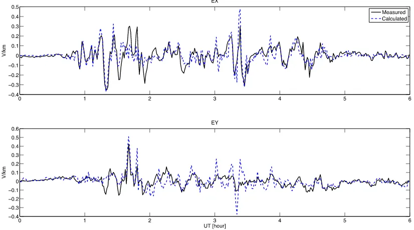
We use the electric field measured during the substorm on 26 June 1998 at stations Jokkmokk and Boden (see Fig. 4) as our test cases. We use the vertical magnetic variations observed at all other BEAR stations (i.e. excluding mag-netic data from the station being studied) as the input data and calculate the surface electric field at Jokkmokk and Bo-den using the SECS technique. Figures 5 and 6 show the measured electric fields and the results of our calculation. For clarity we have plotted 1-minute averages taken from 10-second data. Agreement between the measurement and calculation is very good, except for the x-component at Jokkmokk. The correlation coefficients are−0.22 and 0.82 forx- and y-components at Jokkmokk, and 0.72 and 0.64 for thex- andy-components at Boden, respectively.
horizon-Fig. 5. The measuredx-component (North, upper panel) andy-component (East, lower panel) of the surface electric field at Jokkmokk (66.877◦North, 19.014◦East) during the morning hours of 26.6.1998 and the result calculated using vertical magnetic field from the other BEAR stations.
Fig. 6. Same as Fig. 5 for the surface electric field at Boden (65.636◦North, 21.754◦East).
tal magnetic field), which would mean that very dense mag-netometer network are required. And we must of course keep in mind that we completely neglect the curl-free part of the electric field. At the moment we cannot estimate how significantEcf
h could be in the Fennoscandian area, but it’s
known that in some situations it may affect the surface elec-tric field at considerable distances around conductivity gra-dients (e.g. Fergusonet al., 1990). A more thorough study using detailed magnetotelluric data available from the area (e.g. Korja et al., 2002; Lahti et al., 2005) would be quired, before these issues can be reliably identified and re-solved.
4.
Summary and Discussion
We have demonstrated that it is possible to estimate the geomagnetically induced electric field at the Earth’s surface directly from the time derivative of the vertical magnetic field, without any knowledge of the underlying ground’s electric conductivity. The basic idea is to i) separate the sur-face electric field into curl-free and divergence-free parts, ii) solve the divergence-free part from Eq. (3) and iii) neglect the curl-free part. Step i) can always be done, step ii) is the-oretically exact if we only had perfect knowledge of Br at
approxi-mative and amounts to neglecting the anomalous part of the TM-mode.
Our approach is based on methods developed by Van-ham¨akiet al.(2007) and Vanham¨aki (2011) for ionospheric induction studies. Similar integration of Faraday’s law has been previously used by Becken and Pedersen (2003) and Beckenet al.(2008) in MT studies. However, their primary interest is in the impedance tensor ground conductivity structure, while the surface electric field is a side-product. Moreover, as is usual practice in MT studies, their method works in the frequency/wavenumber domain and assumes quasi-uniform sources. Beckenet al.(2008) show that the TE part of the electric field (corresponding to ourEdf) can be calculated using only magnetic tipper vectors as the in-put data, without knowing the detailed ground conductivity structure or the whole surface impedance tensor. While this method might be useful in hypothetical event analysis, e.g. estimating possible GIC levels in a given network, in many GIC applications a time/space domain approach that makes no assumptions about ionospheric sources is more appro-priate.
Our new solution algorithm for the divergence-free part of the surface electric field is based on the use of external equivalent current, which offers a physics-based way to represent the magnetic variations and associated electric field. It should be noted thatJeq,extare enough to represent the whole vertical magnetic disturbance Br, even if part
of the disturbance is created by internal induced currents. The Spherical Elementary Current Systems method is a convenient way to calculate the equivalent current, as it can be easily adapted to accommodate the the spatial extent and shape of various magnetometer networks. Additionally, the individual elementary systems are simple enough to allow analytical calculation of the electric and magnetic fields.
We note that in the SECS analysis we don’t have to pro-vide any explicit boundary conditions for the surface elec-tric field. However, the implicit and automatically included boundary condition is that the equivalent current does not have any sources outside the analysis area (∇ ×Jeq,ext=0 outside), which means that we neglect the possible Lapla-cian part of the electric field in Eq. (1). This is usually an incorrect assumption, and distant current systems are ex-pected to affect the observedEh, especially near the
bound-aries of the analysis area. However, boundary effects can be reduced by extending the elementary system grid some distance outside the area of interest.
In the present analysis we assume that the curl-free part of the surface electric field is zero, which is equivalent to ignoring the magnetotelluric TM mode. This seems to be a reasonable assumption in many situations, as even the simplified plane wave model with a layered Earth model is able to reproduce GIC with good accuracy (Viljanenet al., 2004). However, in general we expect that the surface electric field may have a significant curl-free part near sharp conductivity gradients, such as ocean-land interfaces. In principle we could attempt to estimate the curl-free part from Eq. (11) or by using previously measured impedance tensor, but that would violate our main goal in this article, which is estimating the electric field using only directly measured magnetic data.
We have tested the new calculation method with an ide-alized electrojet, realistic data-based models as well as ac-tual data from the BEAR network. Results for the WTS model indicates that if we had data from an ideal magne-tometer network, the new SECS-based calculation method would give an almost exact result for the surface electric field. Also the results for the temporary BEAR network are quite accurate. Analysis of the substorm event on 26 June 1998 proves that with magnetic data from the BEAR stations we can calculate the electric field at reference sta-tions. However, a more detailed study is needed to deter-mine how large contribution the presently ignored curl-free electric field (magnetotelluric TM mode) makes to the total large-scale surface electric field in the Fennoscandian re-gion, and how it would affect GIC modeling.
In the electrojet test case results based on the IMAGE data were reasonably accurate. However, in many situa-tions the permanent IMAGE network (at the present config-uration) may be too sparse for the new SECS-based calcu-lation method, as the IMAGE-based results for the smaller scale WTS model were practically useless. This is a disad-vantage compared to several previous methods for estimat-ing the surface electric field, as there are methods that work quite well with IMAGE data (e.g. Viljanen et al., 2004). The main theoretical advantage of the presented method is that there is no need to know the Earth conductivity distri-bution. However, it would appear that in practice it isn’t too hard to obtain a conductivity model that is accurate enough for GIC purposes (Thomsonet al., 2009).
We conclude that the principle of calculating the divergence-free part of the surface electric field from time derivative of the vertical magnetic field is sound, and the method works also in practice. However, at present time practical applications may be somewhat limited as the method seems to require data from a relatively dense and spatially extended magnetometer network. However, a more thorough study is needed to evaluate the practical applicability of the presented method in various situations, taking into account e.g. the spatial extent and distribution of the magnetometer array as well as the role of the curl-free electric field caused by charge accumulation at horizontal conductivity gradients.
Acknowledgments. The work of H. Vanham¨aki was supported by the Academy of Finland (project number 126552). We thank all institutes maintaining the IMAGE magnetometer net-work (http://space.fmi.fi/image/). The BEAR project was partly supported by INTAS (no. 97-1162).
Appendix A.
According to Eq. (9) of Amm and Viljanen (1999), the radial magnetic field of a divergence-free SECS below the current layer (ionosphere) is given by
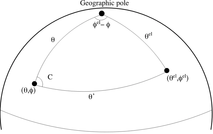
Fig. A.1. Geometry of calculating components of matricesTandS. The elementary system is located at(θel, φel)and the result is evaluated at(θ, φ). θis the co-latitude of the point(θ, φ)in the coordinate system centered at the elementary system.
be solved from Eq. (6)) and θ is the co-latitude of the calculation point expressed in a coordinate system that is centered at the SECS pole. See Fig. A.1 for reference.
The components of the matrix T in Eq. (6) are given simply by
Tn,k=Br,secs(RE, θn,k) /I, (A.2)
where θn,k is the angle between calculation point rn =
(RE, θn, φn)and SECS location relk = (RI, θkel, φkel).
Ac-cording to spherical trigonometry it can be expressed as
cosθn,k=cosθn cosθkel
+sinθn sinθkelcos(φkel−φn). (A.3)
Appendix B.
According to equation (A.6) of Amm and Viljanen (1999), the vector potential of a divergence-free SECS be-low the current layer (ionosphere) is given by
Asecs(r, θ)= μ0
RII
4πrsinθ
1−2rcosθ
RI +
r RI
2
+rcosθ RI
−1
ˆ
eφ. (B.1)
Here the unit vector eˆφ is given in the coordinate system centered at the SECS pole. From Fig. A.1 we can see that in the geographical coordinate system the unit vector can be expressed as
ˆ
eφ= ˆeφcosC+ ˆeθsinC. (B.2)
It is a straightforward exercise in spherical trigonometry to show that
cosC= cosθ
el−cosθcosθ
sinθsinθ (B.3)
sinC =sinθ
elsin(φel−φ)
sinθ . (B.4)
Using Eqs. (A.3–B.4) we can evaluate components of the matrixSfrom expressions
S2m−1,k=Aθ,secs(RE, θm,k) /I, (B.5)
S2m,k=Aφ,secs(RE, θm,k) /I. (B.6)
References
Amm, O., Direct determination of the local ionospheric Hall conductance distribution from two-dimensional electric and magnetic field data: Ap-plication of the method using models of typical ionospheric electrody-namic situations,J. Geophys. Res.,100, 21473–21488, 1995. Amm, O., Ionospheric elementary current systems in spherical coordinates
and their application,J. Geomag. Geoelectr.,49, 947–955, 1997. Amm, O. and A. Viljanen, Ionospheric disturbance magnetic field
contin-uation from the ground to the ionosphere using spherical elementary current systems,Earth Planets Space,51, 431–440, 1999.
Becken, M. and L. B. Pedersen, Transformation of VLF anomaly maps into apparent resistivity and phase,Geophysics,68, 497–505, 2003. Becken, M., O. Ritter, and H. Burkhardt, Mode separation of
magnetotel-luric responses in three-dimensional environments,Geophys. J. Int., 172, 67–86, 2008.
Boteler, D. H. and R. Pirjola, The complex-image method for calculating the magnetic and electric fields produced at the surface of the Earth by the auroral electrojet,Geophys. J. Int.,132, 31–40, 1998.
Boteler, D. H., R. Pirjola, and L. Trichtchenko, On calculating the electric and magnetic fields produced in technological systems at the Earth’s surface by a “wide” electrojet,J. Atmos. Sol.-Terr. Phys.,62, 1311– 1315, 2000.
Chave, A. D. and P. Weidelt, The theoretical basis for electromagnetic induction, inThe Magnetotelluric Method, edited by A. D Chave and A. G. Jones, 552 pp., ISBN 978-0-521-81927-5, Cambidge University Press, Cambridge, 2012.
Egbert, G. D., Processing and interpretation of electromagnetic induction array data,Surv. Geophys.,23, 207–249, 2002.
Ferguson, I. J., F. E. M Lilley, and J. H. Filloux, Geomagnetic induction in the Tasman Sea and electrical conductivity structure beneath the Tasman Seafloor,Geophys. J. Int.,102, 299–312, 1990.
Gilbert, J. L., Modeling the effect of the ocean-land interface on induced electric fields during geomagnetic storms,Space Weather,3, S04A03, doi:10.1029/2004SW000120, 2005.
Gough, D. I., Magnetometer array studies, Earth structure and tectonic processes,Rev. Geophys.,27, 141–157, 1989.
Haines, G. V. and J. M. Torta, Determination of equivalent current sources from spherical cap harmonic models of geomagnetic field variations,
Geophys. J. Int.,118, 499–514, 1994.
Jiracek, G. R., Near-surface and topographic distortions in electromagnetic induction,Surv. Geophys.,11, 163–203, 1990.
Jozwiak, W., Large-scale crustal conductivity pattern in central Europe and its correlation to deep tectonic structures,Pure Appl. Geophys., doi:10.1007/s00024-011-0435-7, 2011.
Korja, T. and the BEAR Working Group, BEAR: Baltic Electromagnetic Array Research,EUROPROBE News,12, 4–5, 1998.
Korja, T., M. Engels, A. A. Zhamaletdinovet al., Crustal conductivity in Fennoscandia—A compilation of a database on crustal conductance in the Fennoscandian Shield,Earth Planets Space,54, 535–558, 2002. Lahti, I., T. Korja, P. Kaikkonen, K. Vaittinen, and BEAR Working Group,
Decomposition analysis of the BEAR magnetotelluric data: implica-tions for the upper mantle conductivity in the Fennoscandian Shield,
Geophys. J. Int.,163, 900–914, 2005.
McKay, A. J. and K. A. Whaler, The electric field in northern Eng-land and southern ScotEng-land: Implications for geomagnetically in-duced currents,Geophys. J. Int.,167, 613–625, doi:10.1111/j.1365-246X.2006.03128.x, 2006.
McLay, S. A. and C. D. Beggan, Interpolation of externally-caused mag-netic fields over large sparse arrays using Spherical Elementary Current Systems,Ann. Geophys.,28, 1795–1805, doi:10.5194/angeo-28-1795-2010, 2010.
Pirjola, R., Geomagnetic effects on ground-based technological systems, inReview of Radio Science 1999–2000, edited by W. R. Stone, 24 pp., ISBN 978-0-471-26866-6, Wiley-IEEE Press, New York, 2002. Pirjola, R. and A. Viljanen, Complex image method for calculating electric
and magnetic fields produced by an auroral electrojet of finite length,
Ann. Geophys.,16, 1434–1444, 1998.
Pulkkinen, A., O. Amm, A. Viljanen, and BEAR Working Group, Iono-spheric equivalent current distributions determined with the method of spherical elementary current systems,J. Geophys. Res.,108, 1053, doi:10.1029/2001JA005085, 2003a.
Pulkkinen, A., O. Amm, A. Viljanen, and BEAR Working Group, Sep-aration of the geomagnetic variation field on the ground into external and internal parts using the spherical elementary current system method,
Earth Planets Space,55, 117–129, 2003b.
Pulkkinen, A., A Thomson, E. Clarke, and A. McKay, April 2000 geo-magnetic storm: Ionospheric drivers of large geogeo-magnetically induced
currents,Ann. Geophys.,21, 709–717, 2003c.
Thomson, A. W. P, A. J. McKay, and A. Viljanen, A review of progress in modelling of induced geoelectric and geomagnetic fields with special regard to induced currents,Acta Geophys.,57, 209–219, doi:10.2478/s11600-008-0061-7, 2009.
Thomson, D. and J. Weaver, The complex image approximation for induc-tion in a multilayered Earth,J. Geophys. Res.,80, 123–129, 1975. Vanham¨aki, H., Inductive ionospheric solver for magnetospheric MHD
simulations,Ann. Geophys.,29, 97–108, 2011.
Vanham¨aki, H., A. Viljanen, and O. Amm, Induction effects on ionospheric electric and magnetic fields,Ann. Geophys.,23, 1735–1746, 2005. Vanham¨aki, H., O. Amm, and A. Viljanen, Role of inductive electric fields
and currents in dynamical ionospheric situations,Ann. Geophys.,25, 437–455, 2007.
Viljanen, A. and R. Pirjola, On the possibility of performing studies on the geoelectric field and ionospheric currents using induction in power systems,J. Atmos. Terr. Phys.,56, 1483–1491, 1994.
Viljanen, A., H. Nevanlinna, K. Pajunp¨a¨a, and A. Pulkkinen, Time deriva-tive of the horizontal geomagnetic field as an activity indicator,Ann. Geophys.,19, 1107–1118, 2001.
Viljanen, A., A. Pulkkinen, O. Amm, R. Pirjola, T. Korja, and BEAR Working Group, Fast computation of the geoelectric field using the method of elementary current systems and planar Earth models,Ann. Geophys.,22, 103–113, 2004.
Wait, J. R. and K. P. Spies, On the image representation of the quasi-static fields of a line current source above the ground,Can. J. Phys.,47, 2731– 2733, 1969.
Weygand, J. M., O. Amm, A. Viljanen, V. Angelopoulos, D. Murr, M. J. Engebretson, H. Gleisner, and I. Mann, Application and validation of the spherical elementary currents systems technique for deriving ionospheric equivalent currents with the North American and Green-land ground magnetometer arrays, J. Geophys. Res., 116, A03305, doi:10.1029/2010JA016177, 2011.
Zhang, P., L. B. Pedersen, M. Mareschal, and M. Chouteau, Channelling contribution to tipper vectors: A magnetic equivalent to electrical dis-tortion,Geophys. J. Int.,113, 693–700, 1993.