FULL PAPER
Temporal resolution of internal magnetic
field modes from satellite data
João Domingos
1,2,3*, Maria Alexandra Pais
1,2, Dominique Jault
3and Mioara Mandea
4Abstract
We aim to obtain a modal decomposition of the internal geomagnetic field. In order to do so, we perform a principal component analysis of two virtual observatory datasets, with 4-month sampling time, from the CHAMP (2001–2009) and Swarm (2014–2017) satellite records. The spatial patterns of well-resolved modes calculated from the three field components all have internal origin as expected for these datasets, except for one Swarm mode. For both datasets, we find that the modes with the shortest timescales have also the smallest length scales as expected from a physical standpoint. Also, the energy ordering of the modes is from the least to the most variable, in agreement with inde-pendent results on the main field data spectrum. This is not achieved in regularised inversions of geomagnetic field data into time-varying spherical harmonic decomposition, where the highest degree terms have also the poorest time resolution. The improved accuracy of Swarm data is reflected in the lower level of the noise variance. Keywords: Geomagnetic field, Virtual observatories, Principal component analysis, Swarm constellation, CHAMP satellite
© The Author(s) 2019. This article is distributed under the terms of the Creative Commons Attribution 4.0 International License (http://creat iveco mmons .org/licen ses/by/4.0/), which permits unrestricted use, distribution, and reproduction in any medium, provided you give appropriate credit to the original author(s) and the source, provide a link to the Creative Commons license, and indicate if changes were made.
Introduction
Over more than a century, the temporal variations of the Earth’s magnetic field have been mainly monitored by continuous recordings in geomagnetic observato-ries. Although the number of observatories has stead-ily increased, their geographic coverage remains highly uneven. To overcome this difficulty, satellite data are now available, albeit for only the past two decades. Recent magnetic field models have been constructed from meas-urements obtained from low Earth orbiting satellites car-rying magnetometers, mainly Ørsted, CHAMP, SAC-C and Swarm. Unfortunately, these satellite missions are short in comparison with the correlation times of the Earth’s core magnetic field (Hulot and Le Mouël 1994). Moreover, there may be gaps related to instrumental failure, or non-consecutive missions. Lack of satellite vectorial data between September 2010 (de-orbiting of CHAMP) and November 2013 (launch of Swarm mis-sion) has contributed to the decrease in spatial resolution
of main field models during that period (Beggan and Whaler 2018).
Most analyses of the variability of the main field have been based on time series of spherical harmonic coef-ficients. Lhuillier et al. (2011) estimated the correlation time of the main non-dipole field at 415/ℓ years where ℓ
is the harmonic degree. In addition to its slow variation, the main magnetic field also has decadal and interannual fluctuations, and satellite data covering the last 20 years can be very useful to investigate this range of periods. Close to 1-year timescale, the contribution of the exter-nal field is present and quite strong and a proper separa-tion is not yet possible. Finally, at the high-frequency end of the main field spectrum, its amplitude is too small to be perceived at observatories and satellites.
The time resolution of series of spherical harmonic coefficients from geomagnetic field models has naturally been investigated as a function of ℓ . Models based on
observatory records had lower time resolution for higher degree ℓ : as an example, Langel et al. (1986) represented
the secular variation from 1903 to 1982 using cubic B-splines with up to six nodes for degrees 1–4 but only one internal node for degrees 5 and 6. The situation has improved with the availability of satellite data, and yet,
Open Access
*Correspondence: [email protected]
3 ISTerre, IFSTTAR, IRD, CNRS, University Savoie Mont Blanc, University Grenoble-Alpes, 38000 Grenoble, France
for degrees 5–8, Gillet (2018) remarks that only signals with periods above about 6 years can be retrieved from time-varying current satellite field models. The time res-olution of satellite field models is better for lower degrees and worse for higher ones (compare the spectrum of the second and third time derivatives of the field in Figure 2 of Lesur et al. (2010)). This is a consequence of the regu-larisation techniques used to produce the models (Finlay et al. 2016). It is noteworthy that the lower variability of fine scale structures in models of the Earth’s magnetic field results from the nature of the inverse modelling and does not reflect the time variability of small scale fea-tures of the actual field. This observation has motivated the development of models of the time-varying Earth’s magnetic field that do not involve a projection of the geo-magnetic potential on spherical harmonics (Olsen and Mandea 2007).
Principal component analysis (PCA), also known as principal orthogonal decomposition [see, e.g. Taira et al. (2017) for a recent overview], is a widely used statistical tool to extract a minimal number of energetic coherent structures from a time sequence of scalar maps. It has the advantage of describing the space-time evolution of a physical quantity as the superposition of a few decor-related components (or modes), a property referred to as dimensionality reduction. It is one among different data-based modal techniques used as a prospective analysis of real or simulated data. Besides, in certain cases, physi-cally meaningful structures displaying the symmetries of underlying source mechanisms may emerge from PCA modes. By directly using records of the geomagnetic field at fixed locations (observatories) to conduct a PCA anal-ysis, it may be possible to extract features—with small length scales and/or short timescales—left aside when constructing spherical harmonic models.
As a matter of fact, PCA analysis has been employed to calculate spatio-temporal patterns of the external com-ponent of the field from geomagnetic observatory data (Balasis and Egbert 2006; Shore et al. 2016), giving only an ancillary role to spherical harmonic modelling. Fur-thermore, PCA may allow for the separation between the internal and the external field (which is key to detect rapid variations of the internal field). The analysis of the geomagnetic field vector requires a slight modification of the standard PCA method in order to ensure that the spatial modes for the three components are each subject to the same time variation. We shall refer to it as vecto-rial PCA. Shore et al. (2016) performed such an analy-sis using ground-based geomagnetic data from 1997 to 2009 keeping only the five quietest days in each month, after removal of internal main field and crustal contri-butions. The different modes that they identified have a clear physical significance. Their mode 1 describes the
magnetospheric ring current and is strongly fluctuating. The mode 2 represents an annual oscillation of the global system of currents and mode 3 describes ionospheric sig-nals with semi-annual period.
The two studies of Balasis and Egbert (2006) and Shore et al. (2016) were concerned with the determina-tion of external magnetic field variadetermina-tions. In the con-text of main field studies, however, global coverage is crucial. This explains why the first attempts at applying the PCA method to the main field have relied on spheri-cal harmonic coefficients as the quantity to be analysed either directly (Chulliat and Maus 2014) or after pro-jection to produce maps of the radial field at the core-mantle boundary (Pais et al. 2015a). Pais et al. (2015a) derived explicitly the mathematical conditions when the two approaches are equivalent. From CHAMP models centred on epochs ranging from 2002 to 2009, Chulliat and Maus (2014) retrieved a standing wave of period about 6 years. Pais et al. (2015a) used the CM4 model for 1960–2002 (Sabaka et al. 2004), which is mainly based on observatory data, to obtain large-scale modes and dis-cuss the relationship between their time evolution and the occurrence of geomagnetic jerks. In these studies, the time variability of the modes increases with their rank, a result that is compatible with the ∼f−4 energy spectrum of the main field (De Santis et al. 2003; Lesur et al. 2018).
Using PCA in the context of dynamical systems theory, to reconstruct the state space of a system from experi-mental time series of some univariate stochastic variable, Gibson et al. (1992) showed that discrete Legendre poly-nomials can very closely approximate the set of orthog-onal basis functions that describe time variation. In a recent study, McKinnon et al. (2016) used explicitly the first four Legendre polynomials to project a data matrix on variability of daily maximum and minimum summer temperatures over the Northern Hemisphere, because they are so similar in shape with the time basis resorting from PCA.
Assuming that over 1 month the external field contribu-tions can be neglected, they estimated the parameters of the residuals and used them to compute a mean magnetic field residual for each VO and each month. The result-ing VO time series correlate well with the correspond-ing ground-based observatories time series (Olsen and Mandea 2007). In contrast with measurements at real ground observatories, VO series are free from local crus-tal effects. Beggan et al. (2009) followed up the approach developed by Mandea and Olsen (2006) and created VO datasets from both Ørsted and CHAMP satellite meas-urements. They found that external fields cannot be entirely removed and produce, as a result, unrealistic sec-ular acceleration of the main field. Saturnino et al. (2018) illustrated an alternative methodology with 2 years of Swarm data. They neither selected the data nor removed a model for the external field. They applied instead an equivalent source dipole technique. They accounted for the recorded magnetic field by an ensemble of time-varying dipoles located at the core-mantle boundary and reconstructed VO series at a uniform altitude from these time-varying dipoles.
We undertake here a PCA analysis of the VO datasets recently created by Barrois et al. (2018). They calculated separate datasets from CHAMP and Swarm measure-ments which are as free as possible from contributions of the external field. Both time series have a time resolution of 4 months with almost no gaps despite strict selection criteria of the magnetic measurements.
The next section (“Data” section) consists in a descrip-tion of the VO datasets. It is followed in “Methods” sec-tion by a summary of the PCA method that we employed. Our main results are presented in “Results” section, where we compare the modes calculated from CHAMP and Swarm data, respectively, and a discussion follows in “Discussion” section, focusing on the issue of time reso-lution. The paper ends by pointing out, in “Conclusions and perspectives” section, the main conclusions and some interesting future developments.
Data
Virtual observatories
Here, we use two sets of recent VO series, similar to the one presented by Barrois et al. (2018) with some small changes including the number of VOs: one of them was calculated from measurements provided by the CHAMP vector magnetometer (from July 2000 to September 2010) and the other one was computed from three Swarm vector magnetometers (from November 2013 to December 2017). For the self-consistency of this paper, let us summarise the applied procedure.
To calculate the magnetic field values at each VO location, firstly a data selection needs to be applied in
order to reduce the noise and aliasing due to the high-frequency currents in the magnetosphere and the iono-sphere, and charges circulating near and across the satellites orbit. The initial dataset consists of CHAMP MAG-L3 and Swarm Level 1b MAG-L, version 0501 at 15-second sampling rate data. Large outliers deviating more than 500 nT from the CHAOS-6-x3 model (Finlay et al. 2016), were removed. The next step in data selec-tion consists in considering only night-time (Sun at most
10◦ above horizon) and geomagnetically quiet conditions
( Kp<30 , |dRC/dt|<3 nT/h, Em≤0.8 mV/m, Bz>0 and |By|<10 nT, where Kp is the geomagnetic activity
index, RC is the ring current disturbance index, Em is
the merging magnetic field at the magnetopause, By and
Bz are components of the interplanetary magnetic field,
see Barrois et al. (2018) for a precise definition of these parameters). For the CHAMP dataset, along-track sums and differences were used, while the Swarm dataset ben-efits from using both along-track and cross-track sums and differences, which provide a signal less perturbed by external sources.
To minimise other possible un-modelled sources, sev-eral processing steps were applied and the contributions from different sources removed from data: (1) the magne-tospheric field (up to degree ℓ=2 ) and its Earth-induced counterpart as given by the CHAOS-6-x3 model; (2) the ionospheric and its induced fields as given by the CM4 model (Sabaka et al. 2004); (3) the time-dependent inter-nal field for spherical harmonic degrees ℓ≤20 and the
static internal field for ℓ >20 given by the CHAOS-6-x3
model. Note that these corrections involve different coor-dinate systems. Both the core and ionospheric fields are estimated in the geographic coordinate system. The fields due to near Earth magnetospheric sources, including the ring current, are calculated in the solar magnetic coor-dinate system (with the z axis defined as the dipole axis, and the Sun-Earth line contained in the xz plane, see, e.g. Laundal and Richmond 2017). The fields due to remote magnetospheric sources are calculated in the geocentric solar magnetic coordinate system (x axis along the Earth-Sun line, dipole axis in the xz plane).
observation points are calculated in a local Cartesian coor-dinate system with the origin at the VO position.
Data selection for PCA
The VOs data from CHAMP satellite and Swarm constella-tion of three satellites were used to perform a PCA analysis of the magnetic field. VO data are provided for a fixed set of spatial coordinates, which is a requirement of PCA decom-position. In order to work with the longest possible simul-taneous series in a fixed number of VOs, the period under study is shorter than the satellite mission periods, from November 2001 to November 2009 for CHAMP and from March 2014 to November 2017 for Swarm. Both datasets consist of vector magnetic field values every 4 months, for a total of 25 epochs for CHAMP and 12 epochs for Swarm. The number of grid points for CHAMP is NP=292 , since
8 of the original VOs presented recurrent gaps.
For Swarm, a different set was constructed, since field values representative of the core field were systematically missing at high latitude VOs, due to strong external per-turbations. For this reason, Swarm dataset consists of only NP =258 VOs between −60◦ and 60◦ latitude (sub-auroral
grid). Same as in Shore et al. (2016), PCA is applied on a data matrix with Br , Bθ and Bφ components (where (r,θ,φ)
are spherical polar coordinates).
Although Swarm data are more precise, the longer time series from CHAMP allows to expect a better resolution of modes that have annual to decadal characteristic time-scales. The equal area distribution of grid points makes it unnecessary to apply a latitudinal weighting factor, which would have been the case for the geographic regular grid spacing approach or for the existing network of ground observatories (Shore et al. 2016). The altitude RVO of the
VOs obtained from CHAMP and Swarm data is 300 km and 500 km, respectively. This slightly complicates the comparison between the modes obtained from the two datasets.
Methods
Implementation of principal component analysis
To apply PCA, geomagnetic data for the spherical field components at M distinct epochs and from a total num-ber NP of VOs are distributed into M×3NP data matrix X . Each row i, say xTi , is the set of 3NP ‘data’ for a certain
epoch i, once the time average has been removed. The set of all rows can be seen as the M realisations of a 3NP
-vari-ate stochastic variable (e.g. Jolliffe 2002):
(1)
Notation and nomenclature follow closely Pais et al. (2015b). By applying PCA, it is expected that a large frac-tion of the variability of the geomagnetic field may be described with a k-variate variable yiT where k≪3NP .
This is achieved by projecting each xiT onto the
eigenvec-tors of the covariance matrix CX =XTX/(M−1):
where the columns ( pj ) of P are the normalised
eigenvec-tors of CX , i.e. pj Tpj=1 . Then, Y=XP is the M×3NP
matrix with rows yiT , and X=YPT since P is orthogonal.
By arranging the columns of P in decreasing order of
cor-responding eigenvalues, the first k elements of yi explain
most of the variability in the data matrix X , meaning that
the data matrix can be reconstructed from the first k col-umns of Y and the first k columns of P:
where yj is column-j of Y , y′j is the corresponding vec-tor normalised to unity ( y′j Ty′j=1 ), αj are non-negative
scalars (the singular values of data matrix X ) and ⊗ is for
dyadic product (see, e.g. Hannachi et al. 2007). In (2), the data matrix has been decomposed into principal com-ponents or modes, each mode-j consisting of the prod-uct of a time series called principal component (PC) (the columns of Y ) and a spatial structure called empirical
orthogonal function (EOF) (the columns of P ). The
indi-ces for mode rank and epoch appear as superscript and subscript, respectively.
How close to X is (2) depends on how many terms we
keep in the expansion, i.e. on k, but also on the intrin-sic nature of the signal. As an example, when apply-ing PCA to the main field (MF), its secular variation (SV) and its secular acceleration (SA) during the time period 1960 to 2002, the first mode in each independ-ent analysis explains over 90% of the MF variance, about 70 % of the SV variance and only 30 % of the SA variance (Pais et al. 2015a). The variance explained by mode-j, describing how variable is the (zero mean) parameter yj among different realisations, is given by M the non-negative real eigenvalue j of covariance matrix
CX once the ordering by decreasing value has been
applied. Note that j and αj in (2) are related through
j=(αj)2/(M −1).
The computation of eigenvectors and eigenvalues of the covariance matrix CX , on which the principal modes rely,
depends on the working sample. The best approximations are sample estimators, for which North et al. (1982) give first-order sampling errors:
where j and l are consecutive modes and n∗ is the number
of degrees of freedom, that takes into account the cor-relation between consecutive samples. In the absence of some a priori on the autocorrelation structure of the time series, the sample size M will be used instead [but see Hannachi et al. (2007) for other possibilities]. According to (3), plotting δj as error bars associated with each j gives information not only on the separation of tive eigenvalues but also eigenvectors. In case consecu-tive j and l are closer than δj , the modes are said to be degenerate and any linear combination of those modes is as significant as each one of them (Hannachi et al. 2007).
Gibson et al. (1992) found that PCs can be identified with discrete Legendre polynomials when some conditions are met. They showed that, in the so-called small-win-dow regime, the temporal orthogonal basis vector yj [see Eq. (2)] is very closely given by Lj , the Legendre polynomial of degree j. Furthermore, the order-j time derivative of the field, taken at the mid-point of the time window, can be approximated as the inner product between Lj and the data series at each VO. In other terms, the consecutive EOFs give a good approximation of the successive time deriva-tives of the field at the mean epoch. The condition that has to be met is that τW ≪τW , where c τW is the dataset
win-dow width and τWc is a critical width that depends on the
relative variance of the two lowest-order time derivatives of the signal. In certain cases, but not always, τWc may be used
as an estimate for the correlation time of the signal [see Gibson et al. (1992)]. The degree-0 Legendre polynomial does not arise here as a principal component because the time average of the field components has been subtracted before the PCA analysis. The two lowest-order derivatives in the remaining signal are order 1 and order 2, which together allow to define the critical time width, using as an approximation to these variances the first two CX
eigenval-ues. From equation (117) in Gibson et al. (1992):
(3)
in the same unit of time as used in the PCA computa-tions, which in our case is year/3 (4 months).
Denoting τW the length of the time series (8 year for
CHAMP and 3.7 year for Swarm), we can associate a time resolution
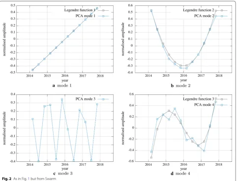
to each principal component close to a Legendre polyno-mial of degree j (i.e. all modes in Figs. 1, 2 but the annual mode from Swarm data).
Spherical harmonic models
The standard decomposition of the Earth’s irrotational field into spherical harmonic functions allows for the internal and external contributions to be parameterised separately. Note that the construction of VOs series does not account for effects due to poloidal electric currents crossing the cylindrical cells, as those coupling the mag-netosphere and the ionosphere (see, e.g. Sabaka et al. 2010). With this approximation, only potential fields can be modelled with internal and external sources defined with respect to VOs, internal if below the VOs altitude and external if above, i.e. B= −∇V with
where RVO is the spherical shell radius at the VOs
alti-tude, Pml are the associated Legendre functions having Schmidt semi-normalisation and (gℓm,hmℓ) and (qℓm,smℓ) are the internal and external spherical harmonic (SH) coefficients at the VOs altitude.
We can also define an average spherical harmonic degree ℓB , weighted by the internal magnetic field energy,
for each mode of CHAMP and Swarm as
B2ℓ is the contribution of internal SH degree-ℓ terms for
the mean energy of the field at the VOs altitude [see Christensen and Aubert (2006) for the analogous defini-tion of the average spherical harmonic degree of the flow in the Earth’s core].
The eccentric dipole approximation
The field can be approximated as a point dipole mov-ing with respect to the Earth’s centre, with its mag-netic moment rotating relative to the geographic frame. Then, the field variation is simulated considering only the eccentric dipole component as given by Schmidt (1934) and Bartels (1936) who imposed the invariance
B2ℓ =(ℓ+1) ℓ
m=0
(gℓm) 2
+(hmℓ)
2
.
of the dipole moment: the eccentric dipole so-defined has the same moment and the same orientation as the centred dipole defined from the three Gauss coef-ficients of degree 1. The position rED of the eccentric dipole (i.e. the offset between the dipole centre and the Earth’s centre) is then chosen to minimise the squared quadrupole moment as seen from rED [see, e.g. Lowes (1994) and references therein]. Bartels (1936) gave the equations used to determine rED [see his equations (14) and (15) reproduced in Fraser-Smith (1987)], which depend only on Gauss coefficients of degrees 1 and 2.
On spheres r=R outside the Earth’s surface and cen-tred at the Earth’s centre, an eccentric dipole located at
rED , with s=rED/R≪1 produces a field dominated
by its components of degree 1 and 2. James and Winch (1967) showed that a dipole of moment Mmˆ located at
rED is equivalent to an infinite sum of centred multipoles,
along mˆ ). The strength of different multipoles scales with degree ℓ as Msℓ−1/(ℓ−1)! , where s∼0.08 for the pre-sent field and at the satellite altitude.
Application of PCA to VO series
Following Shore et al. (2016) who use the three magnetic components at each observatory as additional param-eters of the multivariate variable, we write
with the NP values of the radial component at epoch i
concatenated with the NP values for each of the other two
sets of components. The extracted EOFs have the same structure, i.e. pj T =pj Tr ,pj Tθ ,p
j T
φ
, the 3 components evolving correlated in time according to the time series given by a single PC. Besides, if the xi parameters satisfy
linear constraints such as ∇ ·B=0 and B= −∇V , each
EOF will also satisfy the same constraints. Barrois et al.
xTi =xiT,r,xiT,θ,xTi,φ
(2018) have used these constraints to construct the VO series but locally only, in cylindrical volumes around each VO location. We can thus measure the physical signifi-cance of the different modes by estimating to what extent they satisfy these constraints not only locally but also over the whole spherical surface where VOs are distrib-uted. The potential theory leads us also to discriminate between internal or external sources.
The vectors y′j and pj are adimensional, both
normal-ised to unity. This introduces scaling factors 1/√M and 1/√3NP in the coefficients of y′j and pj , respectively. The
geomagnetic field at each grid point at the satellite alti-tude is recovered from combining the normalised time and space vectors with the scaling factor αj (see Eq. 2),
in nT, such that the singular values αj of data matrix X are related with the eigenvalues j of CX through
αj=√j√M−1 . In the end, the mean value of each
field component at each grid point due to mode-j, in nT, is given by
The PCA method is nonparametric and decomposes the entire magnetic field into separate modes only on the basis of existing correlations in the data. In order to sepa-rate sources into internal and external, standard spherical harmonic analysis was applied to the individual modes produced by the PCA method. We start by considering an internal field model. If such a model fits closely a given mode, this mode will be identified as internal. In contrast, high misfits are interpreted as meaning that the mode is due, at least partly, to external sources. To clarify the geometry of external sources, we also fitted an external model to each main PCA mode. The normalised misfit is obtained from the residuals of the SH model compared to the PCA mode as in Eq. (9)
where pM is the fitted model and pj is the EOF vector of
mode-j.
Results
The PCA is applied to 8 years of CHAMP data, from November 2001 to November 2009, and 44 months of Swarm data, from March 2014 to November 2017, with a sampling interval of 4 months. We have chosen to remove the average field (including the crustal field) prior to calculating the PCA. Keeping it would have introduced the mean field, which is approximately a zonal dipole, as another spatial mode.
Identification of the principal components as Legendre polynomials
The (normalised) time series corresponding to the first four modes from CHAMP are represented in Fig. 1. We discuss them together with the time series for modes 1, 2 and 4 from Swarm (see Fig. 2). It appears that these prin-cipal components are well approximated by polynomials of degree increasing with the mode order.
Using eigenvalues of the covariance matrices from CHAMP and from Swarm VO series, we obtain τWc ∼ 30–70 year from Eq. (4), much larger than each corresponding dataset window τW , of 8 and 3.7 year. A more precise gauge for the small-window regime is
ε=(τW/τWc )2 , that should be kept such that ε≪1 in order that Legendre polynomials may be used as tempo-ral basis functions (Gibson et al. 1992). This condition is verified in our study since ε∼0.01.
We superpose in Fig. 1 the Legendre polynomials of degree 1 to 4 to the principal components of rank 1 to (8)
j
M−1 M
1
√
3NP .
(9) �=
(pM−pj)T(pM−pj),
4 calculated from CHAMP data, all time series normal-ised to unity. Similarly, in Fig. 2, we show the Legendre polynomials of degree 1, 2 and 3 together with the princi-pal components of rank 1, 2 and 4 obtained from Swarm data. The agreement is remarkable even for the compo-nents of rank 4, which we deem not well resolved accord-ing to North’s rule of thumb.
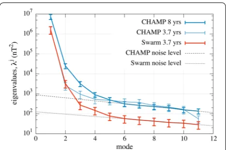
The singular spectrum and the level of noise variance
The singular spectrum (the set of j values) is shown for
each dataset, in Fig. 3. After a rapid decrease, not prop-erly represented neither by an exponential nor a power law, a knee follows and then an asymptotic slightly decreasing trend. This is often referred to as a “plateau” and is attained after only a few modes at a height level that is related to the amplitude of the Gaussian noise in the data (see, e.g. Gibson et al. 1992). For eigenvalues above the plateau, North’s rule of thumb (3) is used to locate the order in the PCA expansion where modes are no longer independently resolved and become degener-ate. This occurs after order 4 for CHAMP and order 3 for Swarm datasets.
Differences between the two spectra in Fig. 3 might be due to different behaviour of the field in the two peri-ods 2001–2009 and 2014–2017, different quality of the two datasets or different sample size, M. From results shown in Figs. 1 and 2, the order-1 PC is a straight line, i.e. y1=α1y′1=a(t−t0) where t0 is the mean epoch for each dataset. Note that, in those two figures, time t is in year/3 (4 months) and the slope is in units of (year/3)−1 . The parameter a is quite similar for the two datasets. In fact, from y′1 plotted in Figs. 1 and 2 and the values of α1 , we obtain aSwarm =1063 nT/year and aCHAMP=1132
Fig. 3 Singular spectra for CHAMP full ( τW=8 year) dataset (thick blue), CHAMP shortened ( τW=3.7 year) dataset (thin blue) and
nT/year, a difference of only 6%. We shall assume that at epochs that are not too far apart, the field rate of change has not significantly varied and that estimates of this rate do not depend on M. Taking into account that all yj have zero mean, the variance represented by the first mode, which is linear in time, scales with τW , the width of the time window, as τW (2 i.e. M2 ). It turns out that this approximate relationship explains well the relative amplitude of this mode calculated from CHAMP or from Swarm data (see Fig. 3). Conversely, eigenvalues (mode variances) in the noise plateau ( j for j6 ) are expected
to be independent on M if they represent a white noise stochastic process. Therefore, the noise plateau does not depend much on the width of the time window. We can directly compare the noise levels for CHAMP and for Swarm data (see the grey lines in Fig. 3) as the number of CHAMP and Swarm VOs is almost the same. Estimated in nT, we find that the height of the noise level for Swarm data is about 0.4 times the value for CHAMP data.
Figure 3 also shows results of a test where we compare the PCA spectra using the full CHAMP dataset (8 years) with that using only the first 3.7 years, the same length as the Swarm dataset (see the thinner solid line). This nicely supports the previous assumption that the plateau level is independent of M. It also reproduces the predicted varia-tion in 1 . Finally, this test illustrates that more and more modes are resolved as the time window is extended: the amplitude of the resolved polynomial modes increases, while the noise level remains constant.
Assuming that the time series sample analytical func-tions, Gibson et al. (1992) found that the variance of the modes decreases exponentially with their order in the small-window regime. Figure 3 for CHAMP data shows a different law for the decrease of the eigenvalues of the first modes. It should be noted however that the geomag-netic field measurements are arguably better described as realisations of a stochastic process (e.g. Hellio et al. 2014) rather than as values taken by an infinitely deriv-able function. It would thus be interesting to learn how the eigenvalues in the singular spectrum are expected to decrease when the signal samples the solution of a sto-chastic differential equation.
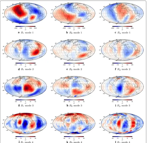
Internal and external modes from resolved empirical orthogonal functions
Figure 4 shows the spatial features of the first four modes of the PCA decomposition of CHAMP VOs. The vector PCA decomposition implies that each mode is charac-terised by three different plots, one for each Br , Bθ and
Bφ components. In order to recover the spatial
distribu-tion of scaled values for a given mode, over time, values in charts of Figs. 4 and 5 have simply to be multiplied by corresponding time series in Figs. 1 and 2 [see Eq. (2)].
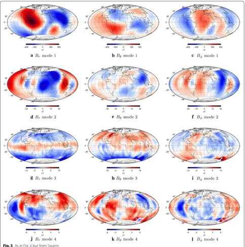
In Fig. 5, we show four distinct modes for Swarm, three of them with temporal variations very similar to CHAMP and mode 3 with a much shorter period of 1 year. The grid for Swarm VOs has less representation in the auroral latitudes, due to very intense external fields there, so we do not show the EOFs at these latitudes.
Table 1 shows the results for these calculations. The three first CHAMP modes and the two first Swarm modes are well explained as internal potential fields. Swarm mode 3, which is dominantly axial quadrupole, shows the lowest misfit when compared to an external model. It consists of both internal and external fields. The misfits between the fourth modes of CHAMP and Swarm and an internal field model are twice as small as their misfits to an external field model. This supports the assessment that they are mainly from internal origin.
Spatial resolution of the successive modes
We represent in Fig. 6, for all modes, their average degree
ℓB , which is directly related to a length scale, as a
func-tion of their time resolufunc-tion, estimated from the degree of the appropriate Legendre polynomial. The time reso-lution TB cannot be directly identified with a charac-teristic timescale as it clearly depends on the length τW
of the time series; the time TB cannot exceed τW . As an example, both modes 1 from CHAMP and Swarm cor-respond to the secular variation of the field, which has a typical timescale much longer than the duration of the satellite records. We nevertheless observe that, glob-ally, ℓB increases as TB decreases: the smallest features of the field have the shortest timescales as expected from a physical standpoint (Nataf and Schaeffer 2015). This con-clusion rests heavily on modes that we do not trust so much, as indicated by the size of the symbols (the larger the symbol, the least the agreement with an internal field model). The strongest evidence yet comes from the com-parison between the first two Swarm modes.
Discussion
Main PCA mode well explained as the variation of the eccentric dipole
Denoting ri the Cartesian coordinates of each VO in
the geographic frame, we calculate the Cartesian coor-dinates in the eccentric dipole frame (see “The eccentric dipole approximation” section), rf , as
where R is the rotation matrix transforming the Earth’s
axis into the magnetic dipole axis. The degree 1 and 2 coefficients of the CHAOS-6 model (Finlay et al. 2016)
(10)
rf =R(ri−rED)
suffice to obtain the dipole moment, the offset rED and
the matrix R at all times. With this, we can transform the
coordinates of the VOs grid of points into the reference frame of the eccentric dipole. We then compute vector components of an axial dipole field at each grid point. Finally, these components are rotated back to the geocen-tric frame and represented at the VOs locations ri.
Figure 7 shows the secular variation due to the eccen-tric dipole evolution calculated from the CHAOS-6
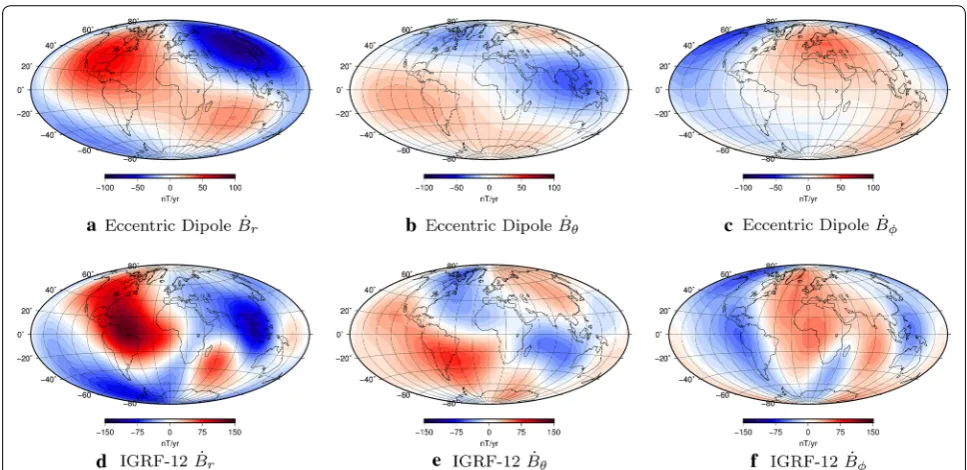
model on the top (difference between the field obtained at consecutive epochs) for epoch 2014, and on the bot-tom we show the secular variation computed directly from the IGRF-12 model, for 2015–2020. The spatial sig-nature we obtain for the moving eccentric dipole asso-ciated secular variation is clearly similar to the spatial pattern of mode 1 and to the IGRF-12 model.
The spatial structures of the first mode recovered from the CHAMP and Swarm datasets are very similar. In fact, using the trend and spatial structure of PCA mode 1
computed from CHAMP dataset, we can explain 60% of the magnetic field signal in Swarm dataset. That is,
where XSwarm is the data matrix from Swarm, (yCHAMP1 ,
p1CHAMP) are the PC and EOF for PCA mode 1 computed using CHAMP dataset and AF denotes the
Frobe-nius norm of matrix A . Had we used PCA mode 1 from
Swarm dataset, we would increase the explained signal in
�XSwarm−yCHAMP1 ⊗p1CHAMP�T F
�XSwarm�F ∼
XSwarm to 70%. This level of predictability can meet the
needs of some fields of study where only the large-scale (or long-distance) component of the main field is impor-tant. It is the case of studies on low Earth orbit satellites vulnerability to energetic particle flux (Domingos et al. 2017). It can also be the case of magnetospheric stud-ies where models for electrical current systems take into account the large-scale main field (e.g. Tsyganenko and Sitnov 2005).
PCA mode 1 gives the average secular variation dur-ing the time interval of CHAMP and Swarm datasets. As a result, it compares well with the IGRF models for these time periods (Thébault et al. 2015).
Higher order time derivatives
The direct reading of computed PCs as Legendre poly-nomials of increasing degree is valid only while in the small-window-width regime, which applies to our data-sets, for which τW << τW . If c τW increases to the point that it gets close to or even larger than τWc , PCs must be
interpreted in a different way. Often, when using PCA on data matrices as (1), the computed PCs are expected to reveal characteristic timescales of the physical mecha-nisms contributing to those particular datasets. As an example, Domingos et al. (2017) retrieved a quasi-perio-dicity of ∼ 11 year when applying PCA to the flux of high energy particles over the South Atlantic Anomaly, due to the solar forcing of the neutral atmosphere density. In
Fig. 6 Average SH degree ( ℓB ) of each mode from CHAMP and
Swarm as a function of the time resolution ( TB ). Size of symbols is proportional to the misfit to an internal field model (Table 1) and numbers next to symbols represent the mode ordering
Fig. 7 (Top) Secular variation due to translation and rotation of the eccentric dipole, for the first half of 2014 at 500 km altitude, using CHAOS-6 to compute the ED parameters. (Bottom) Secular variation computed from the IGRF-12 model (2015–2020). Both represented as B˙r , Bθ˙ and B˙φ in nT/ year
Table 1 Normalised misfit values comparing PCA modes with internal and external SH models, for CHAMP and Swarm
Satellite Model Misfit
Mode 1 Mode 2 Mode 3 Mode 4
the same way, if the VOs global signal includes a compo-nent due to a distinct source and with a correlation time short with respect to τW , we expect that PCA succeeds
in extracting it, if its energy rises above the noise level. This is in fact what occurs in the mode 3 from Swarm database.
The second modes resolved in both CHAMP and Swarm datasets may be regarded as Secular Accel-eration (SA) modes. Their importance comes from the fact that SA is seen as a window on the Earth’s core dynamics, since it is mainly the result of the interaction between the flow acceleration and the field, and flow acceleration is read in terms of contributing force terms (e.g. Aubert 2018). The corresponding PCs are very close to the discrete Legendre polynomial of degree-2 (see Figs. 1b, 2b), which is precisely the required fil-ter to calculate the second time derivative of the geo-magnetic field. The spatial-time information retrieved through these modes allows for the characterisation of the components of the SA field, at the mean epoch of each dataset. In agreement with this interpretation, the EOF2 chart in Fig. 4d–f at 300 km altitude (mean epoch 2005.8), is very similar to the chart of SA at the Earth’s surface for 2006 as given by Chulliat and Maus (2014) (see their Figure 7, also built from CHAMP data). It is dominated by spatial structures of SH degree 3 (as expected from our Fig. 6). The secular accelera-tion at the Earth’s surface evolves rapidly and the whole process wherein the Atlantic equatorial patches of SA radial field change from one sign to the other takes about 4 year [see again Figure 7 of Chulliat and Maus (2014)]. This suggests that τW from Swarm may be too
small to properly resolve this mode and could explain why EOF2 is quite different between the two datasets (compare Figs. 4d–f, 5d–f), with a correlation coeffi-cient of only 0.47. Almost the same correlation (0.46) can be found between mode 2 from Swarm and mode 3 from CHAMP, despite the time series corresponding to different order time derivatives.
Modes 2 and 3 from CHAMP have similar average SH degree ℓB (in contrast with the typical increase of ℓB with
the order of the mode), and they are quite similar, up to a longitude shift. The amplitude of mode 3 is higher than predicted from the power law scaling put forward by Gibson et al. (see “The singular spectrum and the level of noise variance” section); yet, it is smaller than the amplitude of mode 2 (see Fig. 3) and the two modes cannot be simply combined to form a propagating wave. Their similarity is nevertheless intriguing, and we can wonder whether it hints at a non-stochastic time pattern, which might be compared, for example, to the geomag-netic oscillation (of period about 6 years) reported by Silva et al. (2012) in the Earth’s surface SA, mostly from
the CM4 model (from 1960 to 2002.5). Other workers have searched too for periodic signals in the SA but at the core-mantle boundary (CMB) instead of the Earth’s surface. Chulliat and Maus (2014) reported a stand-ing wave, of dominant degree ℓ=6 at the CMB and of
period about 6 years, in part of the equatorial belt from a principal component analysis of CHAMP data projected at the core surface [see also Chulliat et al. (2015)]. It is noteworthy, however, that continuation of the SA from the Earth’s surface r=RE to the CMB r=RC is fraught
with difficulties. It entails amplification by a factor of
(RE/RC)ℓ+2 and gives prominence to higher harmonic
degrees (small scale structures) that have to be filtered out, typically above ℓ=6 . All these studies argue for
SA variability and equatorial symmetry of the radial SA in the Atlantic region equatorial belt. This agrees quite well with the geometry of the two modes 2 and 3 from CHAMP at West Africa (Fig. 4d, g). We now need longer and/or more accurate VO series to decide whether these two modes are really interconnected in the description of the same wave-like structure of the field, or if otherwise they do not differ significantly from the expectation of the stochastic null hypothesis producing the f−4 spec-trum of the main field [see Dommenget (2007) for the discussion of such a null hypothesis and the perspectives for future work outlined in “Conclusions and perspec-tives” section].
A f−4 spectrum for the main field corresponds to a f0 spectrum for the secular acceleration, i.e. to a vanishing SA correlation time τSA , but this time has also been
esti-mated from the ratio between SV and SA energy for each degree ℓ separately (Lesur et al. 2008). Computed values
from geomagnetic field models give τSA∼ 10–20 year,
independently of the SH degree (up to ℓ∼10 above
which τSA increases steeply). A similar value is obtained
from the output of geodynamo simulations up to ℓ∼10
above which τSA rapidly decreases (Christensen et al. 2012;
Aubert 2018). From this perspective also, the window length τW of the series that we have analysed is too short.
If modes 2 and 3 from CHAMP were not both related in building a deterministic structure, then the resolved mode 3 could still be read as the third-order time deriva-tive of the geomagnetic field around the mean epoch 2005. It has a relatively large characteristic length scale
ℓB∼3 , with two main radial flux patches over Brazil
and West Africa, at southern low latitudes. It imparts a special high time variability to SA in the near-equatorial region and in particular to the SA radial flux patch over West Africa which remains equatorially symmetric over time.
seen in the EOF charts. In particular, the anti-symmetry over the Americas in Br (Figs. 4g, 5j) and the diagonally
symmetric patches over Central America and South Africa in Bθ (Figs. 4h, 5k), both stand out. In the Swarm
dataset, this mode is not so well resolved and shows some degree of degeneracy (see Fig. 3).
Among all modes resolved by our PCA analysis, it remains to discuss mode 4 from CHAMP. It shows simi-larities to mode 2 (from CHAMP) but displays higher variability close to geomagnetic polar regions, possibly due to the superposed effect of external currents.
Modes of order higher than four remain unresolved below the noise level (see Fig. 3). We can expect that if we had access to longer series, we would retrieve from the PCA decomposition extra terms for the series of Leg-endre polynomials, with better definition.
Annual oscillation mode from Swarm
Mode 3 from Swarm shows a spatial structure pulsating with an approximately annual period, clearly pointing to a magnetic source influenced by the sun. Although the VO series have been cleaned as much as possible from the magnetic fields with sources in the ionosphere and the magnetosphere, there is thus some residual exter-nal sigexter-nal remaining in the Swarm VO series. The spa-tial structure of mode 3, namely its radial component (Fig. 5g), is clearly distinct from the geometry of other EOFs since it is mostly symmetric about the rotation axis (more precisely, the geomagnetic dipole axis). It shows a band around the geomagnetic equator, charac-teristic of a zonal quadrupolar geometry (resulting from a P20(cosθ ) term in the magnetic potential, see Eq. 6, in the geomagnetic dipole reference frame). Mode 3 from Swarm cannot be due to a solenoidal field of internal ori-gin (relative to the VOs altitude) since the misfit to an internal potential field reported in Table 1 is high. Nei-ther is it a solenoidal field completely external to the VO locations. Thus, contributions from both internal (iono-sphere, induced fields in the crust and mantle) and exter-nal (magnetosphere) sources are present. Outside the auroral regions, which are not represented in our study, we report deviations reaching ±2.6 nT (obtained by
mul-tiplying the time series in Fig. 2c by charts in Fig. 5g, see Eq. (2)). This value is much reduced compared to ampli-tudes between 10 and 20 nT for Malin and Isikara (1976) and Shore et al. (2016). It thus appears that much of the annual oscillation has been removed from the VO series.
The annual oscillation observed at the Earth’s surface (Malin and Isikara 1976), before any treatment to mini-mise it, also presents a dominant quadrupolar struc-ture. However, the geographic coordinate system used in Malin and Isikara (1976) and in the present study is arguably not the most appropriate system to represent
magnetic fields with sources in the magnetosphere. As a matter of fact, Shore et al. (2016) calculated EOFs in the solar magnetic system to make the external field as static as possible in their chosen reference frame. They nevertheless also detected an annual oscillation and interpreted it as the result of a North-South oscillation of the system of external currents arising from the sea-sonal motion of the Sun in the solar magnetic coordinate system. Shore et al. (2016) showed the annual oscillation (see their Figure 6b) as a function of the magnetic local time defined in this coordinate system. They did not state whether the signal would be static in the geocentric solar magnetic system used by Barrois et al. (2018) to calcu-late, in addition to the solar magnetic system, some of the external field subtracted from the VO series. Transfor-mation between the solar magnetic system and the geo-graphic coordinate system involves longitudinal averages that explain well the dominantly axial structure of the mode 3 that we obtained from Swarm data.
Even though the CHAMP dataset covers a larger time window, we have found a well-resolved annual mode in Swarm series only. In Fig. 3, the plateau height associated with the noise level decreases from CHAMP to Swarm from about 8.9×10² to 1.3×10² nT2 . The noise level
in Swarm has decreased below the annual mode energy level allowing it to appear as a resolved mode. In fact, the annual mode can also be found in CHAMP but at rank 6–7, with amplitude well below the noise level. These two modes (6 and 7) have a correlation factor of 0.549 and 0.528, respectively, with the annual mode from Swarm (mode 3).
Finally, the 4-month resolution is rather long compared to the 1-year period of the mode discussed in this sec-tion. At an intermediate stage of this study, we examined VO series with monthly resolution. We found again a mode with annual periodicity and similar geometry as the mode investigated here.
Conclusions and perspectives
This study is an effort to retrieve new information on the Earth’s main magnetic field from recent geomagnetic data. We showed that PCA is an interesting alternative to the widely used SH by decomposing the signal into decorrelated modes. PCA seems to more easily retrieve a behaviour where the most rapid oscillations come from the smallest scale features, which is expected on a physi-cal ground.
modes of internal origin from CHAMP data and two from Swarm data. The time series of these modes (PCs) can be represented by Legendre polynomials of increas-ing degree. The correspondence between the principal components of rank 4 with Legendre polynomials and the partial success of the modelling of the associate EOFs as internal potential fields give us also some confidence in the interpretation of the modes of rank 4 obtained from CHAMP and Swarm. Finally, from Swarm data only, we observe a mode with an annual period and quadrupolar geometry of the radial component (mode 3).
We found some interesting features in our results that can be further exploited. We also identified new prob-lems to be tackled.
• The spatial structure of an eccentric dipole mov-ing towards Asia with amplitude increasmov-ing linearly in time is a good approximation to the SV of the main field at first order. After an interval of about 10 years between ∼ 2005 and ∼ 2015 (from mean epoch of CHAMP to mean epoch of Swarm), mode 1 from CHAMP still explains 60% of the time vari-ability of the field during the Swarm period.
• We found that the mode 3 obtained from CHAMP data is well resolved. It corresponds to the third-order time derivative at the middle epoch of the CHAMP series (November 2005). Once fitted into a spherical harmonic model, the mode can be down-ward continued to the CMB taking care to mini-mise the amplification of small scale noise. Inter-preting the magnetic field changes with the radial induction equation at the core surface, we can undertake the estimation not only of the surface flow velocity and of the flow acceleration but also of the second-order time derivative of the velocity. This is all the more interesting as recent studies dif-fer in their estimation of the core flow acceleration over the period 2000–2016. Livermore et al. (2017) found that a high latitude non-axisymmetric jet has dramatically increased over this period, by a factor 3, whereas Barrois et al. (2018) found a much more modest intensification.
• Dommenget (2007) suggested evaluating data-derived EOF modes against modes synthesised from a stochastic null hypothesis. He argued that a spatial first-order autoregressive process (AR1) can be used as the null information for the spatial struc-ture of the climate variability. Similarly, we may use a temporal second-order autoregressive process (AR2) as the null hypothesis for the magnetic field variability (based on the f−4 magnetic energy
spec-trum). Dommenget (2007) showed EOF modes for realisations of the two-dimensional AR1 stochastic
process and introduced the idea of distinct EOFs, i.e. the modes that are the most distinguished from the modes of the null hypothesis. We may use the same approach, now in the time domain, to search for principal components associated with waves in the core, especially the torsional oscillations with about 6 years period (Gillet et al. 2010).
Let us focus on changes brought by Swarm mission and future work related to them:
• In our tests, we found that we need a VO series of length at least 1.67 year to retrieve the annual mode from Swarm [see also Domingos et al. (2017) for an example where the 11-year solar cycle is extracted from a 16.5-year-long series]. Using the same ratio between the length of the time series and the period of the mode, we tentatively suggest that we need at least 10 years of high-quality data to retrieve the mode associated with torsional oscillations in the core, which is expected to reach amplitude of ∼2 nT/
year at Earth’s surface (Cox et al. 2016).
• VOs were devised in order to monitor the internal field and as such the emergence among the EOFs of an annual mode originating from external sources was unexpected. There remains in the VO series a signal arising from external sources with a significant amplitude of about 2 nT. The presence of this signal points to the need of improvements in the calculation of VO series. This effort could benefit from using, as a guide, mode 3 from Swarm that we computed here.
Although the small lifetime of Swarm mission does not yet allow to resolve completely SA features, if the char-acteristic times are indeed ∼ 10 year, the noise variance level has already been reduced possibly due to cross-track sums provided by the constellation of three sat-ellites. This brings some expectation concerning the retrieval of main field modes of smaller variance. But it also calls attention to the need to improve external field models in order to better clean VO series from external contributions.
Authors’ contributions
JD carried out all computational tasks, made figures and wrote first draft of manuscript. AP supervised the work of JD in particular the implementation of PCA and exploitation of results. DJ worked on the interpretation of results and perspectives. MM provided expert advice with geomagnetic field data. All authors discussed the results, participated in the writing and commented on the manuscript. All authors read and approved the final manuscript.
Author details
Acknowledgements
We want to thank Chris Finlay and Magnus Hammer for providing the Virtual Observatory datasets used in this work, and Nicolas Gillet for reading a draft of this paper and making useful comments.
Competing interests
The authors declare that they have no competing interests.
Availability of data and materials
The datasets supporting the conclusions of this article are available in the figshare repository: https ://doi.org/10.6084/m9.figsh are.70683 05.v1.
Funding
This work has been carried out with financial support for JD by CNES (Centre National d’Études Spatiales, France) and “UC - Universidade de Coimbra (DPA-56-16-382)”. CITEUC is funded by FCT - Foundation for Science and Technol-ogy (UID/Multi/00611/2013) and COMPETE 2020 - Operational Programme Competitiveness and Internationalization (POCI-01-0145-FEDER-006922).
Publisher’s Note
Springer Nature remains neutral with regard to jurisdictional claims in pub-lished maps and institutional affiliations.
Received: 18 September 2018 Accepted: 31 December 2018
References
Aubert J (2018) Geomagnetic acceleration and rapid hydromagnetic wave dynamics in advanced numerical simulations of the geodynamo. Geophys J Int 214:531–547
Balasis G, Egbert GD (2006) Empirical orthogonal function analysis of magnetic observatory data: further evidence for non-axisymmetric magnetospheric sources for satellite induction studies. Geophys Res Lett 33:L11311
Barrois O, Hammer MD, Finlay CC, Martin Y, Gillet N (2018) Assimilation of ground and satellite magnetic measurements: inference of core sur-face magnetic and velocity field changes. Geophys J Int 215:695–712 Bartels J (1936) The eccentric dipole approximating the earth’s magnetic
field. Terr Mag Atmos Elect 41:225–250
Beggan CD, Whaler KA (2018) Ensemble Kalman filter analysis of magnetic field models during the CHAMP-Swarm gap. Phys Earth Planet Inter 281:103–110
Beggan CD, Whaler KA, Macmillan S (2009) Biased residuals of core flow models from satellite-derived ‘virtual observatories’. Geophys J Int 177:463–475
Christensen UR, Aubert J (2006) Scaling properties of convection-driven dynamos in rotating spherical shells and application to planetary magnetic fields. Geophys J Int 166:97–114
Christensen UR, Wardinski I, Lesur V (2012) Timescales of geomagnetic secular acceleration in satellite field models and geodynamo models. Geophys J Int 190:243–254
Chulliat A, Maus S (2014) Geomagnetic secular acceleration, jerks, and a localized standing wave at the core surface from 2000 to 2010. J Geo-phys Res Solid Earth 119:1531–1543
Chulliat A, Alken P, Maus S (2015) Fast equatorial waves propagating at the top of the Earth’s core. Geophys Res Lett 42:3321–3329
Cox G, Livermore PW, Mound J (2016) The observational signature of mod-elled torsional waves and comparison to geomagnetic jerks. Phys Earth Planet Inter 255:50–65
De Santis A, Barraclough DR, Tozzi R (2003) Spatial and temporal spectra of the geomagnetic field and their scaling properties. Phys Earth Planet Inter 135:125–134
Domingos J, Jault D, Pais MA, Mandea M (2017) The South Atlantic Anomaly throughout the solar cycle. Earth Planet Sci Lett 473:154–163 Dommenget D (2007) Evaluating EOF modes against a stochastic null
hypothesis. Clim Dyn 28:517–531
Finlay CC, Olsen N, Kotsiaros N, Gillet N, Tøffner-Clausen L (2016) Recent geomagnetic secular variation from Swarm and ground observatories
as estimated in the CHAOS-6 geomagnetic field model. Earth Planets Space 68:112. https ://doi.org/10.1186/s4062 3-016-0486-1
Fraser-Smith AC (1987) Centered and eccentric geomagnetic dipoles and their poles, 1600–1985. Rev Geophys 25:1–16
Gibson JF, Doyne Farmer J, Casdagli M, Eubank S (1992) An analytic approach to practical state space reconstruction. Physica D 57:1–30 Gillet N (2018) Spatial and temporal changes of the geomagnetic field:
insights from forward and inverse core field models. In: Geomagne-tism, aeronomy and space weather: a journey from the earth’s core to the sun, chapter 9, IAGA
Gillet N, Jault D, Canet E, Fournier A (2010) Fast torsional waves and strong magnetic field within the Earth’s core. Nature 465:74–77
Hannachi A, Jolliffe IT, Stephenson DB (2007) Empirical orthogonal func-tions and related techniques in atmospheric science: a review. Int J Climatol 27:1119–1152
Hellio G, Gillet N, Bouligand C, Jault D (2014) Stochastic modelling of regional archaeomagnetic series. Geophys J Int 199:931–943 Hulot G, Le Mouël J-L (1994) A statistical approach to the Earth’s main
mag-netic field. Phys Earth Planet Inter 82:167–183
James R, Winch DE (1967) The eccentric dipole. Pure Appl Geophys 66:77–86
Jolliffe IT (2002) Principal component analysis, 2nd edn. Springer, New York Langel RA, Kerridge DJ, Barraclough DR, Malin SRC (1986) Geomagnetic
temporal change: 1903–1982, a spline representation. J Geomag Geoelectr 38:573–597
Laundal K, Richmond AD (2017) Magnetic coordinate systems. Space Sci Rev 206(1–4):27–59
Leopardi P (2006) A partition of the unit sphere into regions of equal area and small diameter. Electron Trans Numer Anal 25:309–327
Lesur V, Wardinski I, Rother M, Mandea M (2008) GRIMM: the GFZ Reference Internal Magnetic Model based on vector satellite and observatory data. Geophys J Int 173:382–394
Lesur V, Wardinski I, Hamoudi M, Rother M (2010) The second generation of the GFZ Reference Internal Magnetic Model. Earth Planets Space 62:765–773. https ://doi.org/10.5047/eps.2010.07.007
Lesur V, Wardinski I, Baerenzung J, Holschneider M (2018) On the frequency spectra of the core magnetic field Gauss coefficients. Phys Earth Planet Inter 276:145–158
Lhuillier F, Fournier A, Hulot G, Aubert J (2011) The geomagnetic secular-variation timescale in observations and numerical dynamo models. Geophys Res Lett 38:L09306
Livermore PW, Hollerbach R, Finlay CC (2017) An accelerating high-latitude jet in Earth’s core. Nat Geosci 10:62–68
Lowes FJ (1994) The geomagnetic eccentric dipole: fact and fallacies. Geo-phys J Int 118:671–679
Malin SRC, Isikara AM (1976) Annual variation of the geomagnetic field. Geophys J R Astron Soc 47:445–457
Mandea M, Olsen N (2006) A new approach to directly determine the secular variation from magnetic satellite observations. Geophys Res Lett 33:L15306
McKinnon KA, Rhines A, Tingley MP, Huybers P (2016) The changing shape of Northern Hemisphere summer temperature distributions. J Geophys Res Atmos 121:8849–8868
Nataf HC, Schaeffer N (2015) Turbulence in the core. In: Schubert G (ed) Treatise on geophysics, chapter 8.06, vol 8. Elsevier, Oxford North GR, Bell TL, Cahalan RF, Moeng FJ (1982) Sampling errors in the
estimation of empirical orthogonal functions. Mon Weather Rev 110:699–706
Olsen N, Mandea M (2007) Investigation of a secular variation impulse using satellite data: the 2003 geomagnetic jerk. Earth Planet Sci Lett 255:94–105
Pais MA, Alberto P, Pinheiro FJG (2015a) Time-correlated patterns from spherical harmonic expansions: application to geomagnetism. J Geo-phys Res Solid Earth 120:8012–8030
Pais MA, Morozova AL, Schaeffer N (2015b) Variability modes in core flows inverted from geomagnetic field models. Geophys J Int 200:402–420 Sabaka TJ, Olsen N, Purucker E (2004) Extending comprehensive models of
the Earth’s magnetic field with Ørsted and CHAMP data. Geophys J Int 159:521–547
Handbook of geomathematics, chapter 43. Springer, New York, pp 503–538
Saturnino D, Langlais B, Amit H, Civet F, Mandea M, Beucler E (2018) Com-bining virtual observatory and equivalent source dipole approaches to describe the geomagnetic field with Swarm measurements. Phys Earth Planet Inter 276:118–133
Schmidt A (1934) Der magnetische Mittelpunk der Erde und seine Bedeu-tung. Gerlands Beitr Geophys 41:346–358
Shore RM, Whaler KA, Macmillan S, Beggan C, Velímský J, Olsen N (2016) Decadal period external magnetic field variations determined via eigenanalysis. J Geophys Res Space Phys 121:5172–5184
Silva L, Jackson L, Mound J (2012) Assessing the importance and expres-sion of the 6 year geomagnetic oscillation. J Geophys Res Solid Earth 117:B10101
Taira K, Brunton SL, Dawson STM, Rowley CW, Colonius T, McKeon BJ, Schmidt OT, Gordeyev S, Theofilis V, Ukeiley LS (2017) Modal analysis of fluid flows: an overview. AIAA J 55:4013–4041
Thébault E, Finlay CC, Beggan CD, Alken P, Aubert J, Barrois O, Bertrand F, Bondar T, Boness A, Brocco L, Canet E, Chambodut A, Chulliat A, Coïs-son P, Civet F, Du A, Fournier A, Fratter I, Gillet N, Hamilton B, Hamoudi M, Hulot G, Jager T, Korte M, Kuang W, Lalanne X, Langlais B, Léger J-M, Lesur V, Lowes FJ, Macmillan S, Mandea M, Manoj C, Maus S, Olsen N, Petrov V, Ridley V, Rother M, Sabaka TJ, Saturnino D, Schachtschnei-der R, Sirol O, Tangborn A, Tøffner-Clausen L, Vigneron P, Wardinski I, Zvereva T (2015) International Geomagnetic Reference Field: the 12th generation. Earth Planets Space 67:79. https ://doi.org/10.1186/s4062 3-015-0228-9
![Fig. 1 Normalised time series y′j [see Eq. (2)] corresponding to the first four modes from CHAMP, in blue, and corresponding normalised Legendre polynomials, in grey](https://thumb-us.123doks.com/thumbv2/123dok_us/876372.1105298/6.595.60.542.87.449/normalised-series-corresponding-champ-corresponding-normalised-legendre-polynomials.webp)