Spatio-Temporal Video Object Segmentation
via Scale-Adaptive 3D Structure Tensor
Hai-Yun Wang
School of Electrical and Electronic Engineering, Nanyang Technological University, Nanyang Avenue, Singapore 639798 Email:[email protected]
Kai-Kuang Ma
School of Electrical and Electronic Engineering, Nanyang Technological University, Nanyang Avenue, Singapore 639798 Email:[email protected].
Received 29 January 2003; Revised 5 September 2003
To address multiple motions and deformable objects’ motions encountered in existing region-based approaches, an automatic video object (VO) segmentation methodology is proposed in this paper by exploiting the duality of image segmentation and motion estimation such that spatial and temporal information could assist each other to jointly yield much improved segmentation results. The key novelties of our method are (1)scale-adaptivetensor computation, (2)spatial-constrainedmotion mask generation
withoutinvoking dense motion-field computation, (3)rigidity analysis, (4) motion mask generation and selection, and (5) motion-constrainedspatial region merging. Experimental results demonstrate that these novelties jointly contribute much more accurate VO segmentation both in spatial and temporal domains.
Keywords and phrases:video object segmentation, 3D structure tensor, rigidity analysis.
1. INTRODUCTION
Due to large amount of data and highly dynamic contents, digital video processing creates many technical challenges for conducting even some basic tasks that we, human beings, have been simply taking for granted in our daily lives. Among these operations,video object (VO) segmentationis an emerg-ing signal processemerg-ing tool, and is gradually becomemerg-ing indis-pensable to many digital video applications often encoun-tered in multimedia, virtual reality, computer vision, and machine intelligence. Given a digital video, how to bestow a machine with the capability of automatically (i.e., unsuper-visedly) segmenting dominant VOs with reasonable accuracy on objects’ boundaries is by no means a small goal.
Various VO segmentation methods [1,2,3,4,5,6,7,8] are proposed to combine image (or spatial) and motion (or temporal) segmentations together to enhance the accuracy of VO extraction. Typical VO segmentation methodologies can be grouped into three categories: (1) region-based [1,2]; (2) boundary-based [3,4,5]; and (3) probabilistic model-based approaches [6,7,8].
Region-basedmethods were developed by performing the clustering operation [1] or regional splitting and growing [2] on the feature space, which is usually formed by mo-tion vectors and some spatial features, like color, texture, and
position. However, accurate region boundary is difficult to achieve. Since human visual system (HVS) is very sensitive to the edge and contour information,boundary-based tech-niques were implemented with this consideration in mind by usingedge detectors[3],level set and fast marching[4], or ac-tive contours[5], further combined with motion-field infor-mation for VO segmentation. Such approaches are very sen-sitive to noise, and the evolution of the active contour highly depends on the given initial position or convergence param-eters imposed by the user.Probabilistic model-based methods exploit Bayesian inference [6], minimum description length (MDL) [7], or expectation maximization (EM) [8] to extract moving objects. Although these approaches are theoretically formulated, they suffer from high computational complexity. Some of them also need the number of objects/regions pre-assumed as an input parameter, which might prohibit their usage in practical applications.
(2)deformable/nonrigidmotion, which is encountered when the VO moves with various changes in sizes and shapes dur-ing a scene of the video sequence. How to performrigidity analysis is important to yield accurate motion models for capturing objects’ individual characteristics.
To address the above-mentioned two problems en-countered in VO segmentation, a novel VO segmentation methodology is proposed in this paper that integrates spa-tial and temporal information in a similar way to what are performed in the HVS cortex’s pathways. The novelty of our method is that we only use the eigenvalues of the lo-cal three-dimensional (3D) structure tensor without com-puting dense motion vectors; thus, our method yields much lower computational load and is less sensitive to noise and global/background motion [9]. Furthermore, in the calcu-lation of the 3D structure tensor, thescale-adaptive spatio-temporal Gaussian filter is introduced to handle multiple VOs under different motions in which thescale(i.e., the win-dow size) is driven by the condition number. To diff eren-tiate whether the sequence contains rigid or nonrigid mo-tion, rigidity analysis is performed using correlation coeffi-cients over a range of successive video frames. The largest eigenvalue and coherency measurements of the 3D structure tensor are computed to form motion masks (i.e.,eigenmap andcorner map, respectively), which are further selected by thechange detectionand refined by graph-based spatial seg-mentation for rigid and nonrigid motions, respectively. And, for the final spatial VO segmentation, region merging is per-formed on adjacent over-segmented spatial segments based on the thresholding of the distance computed between the 3D structure tensor and an affine motion model [10]. Such a parametric method results in much more relevant VO seg-mentation and accurate VO boundaries as compared to en-ergy minimization approach [11].
The paper is outlined as follows.Section 2highlights the main ideas of our methodology.Section 3introduces the ba-sics of the 3D structure tensor and provides an overview of existing methods relevant to our work. Section 4describes our proposed VO segmentation methodology. Experimental results of our scheme and comparison with other approaches are presented inSection 5. Finally, conclusions are drawn in
Section 6.
2. FOUNDATION
2.1. The duality of image segmentation and motion estimation
In the previous works, several image segmentation [12] and motion segmentation [10, 13] techniques have been pro-posed for extracting the moving VOs. Image segmentation is to partition an image into nonoverlapping regions so that each one is “homogeneous” in some sense, such as intensity, color or, texture. The most commonly-used segmentation techniques can be classified into two broad categories [12]: (1) region-based segmentation that looks for regions satisfy-ing a given homogeneity criterion; and (2) boundary-based segmentation that looks for boundaries between adjacent
re-gions whose characteristics are different. Generally speak-ing, image segmentation techniques can produce good re-sults among homogeneous regions with distinct boundaries (e.g., cartoon images), in which the produced segments are assumed to be piecewise constant/smooth. However, region-based techniques often fail to yield the desired region bound-aries due to the difficulty of choosing a reasonable starting “seed” for region growing and appropriate growing/stopping rules. Moreover, boundary-based techniques are sensitive to noise and tend to be trapped into local minimum points like small edges.
Two main methods of motion estimation used formotion segmentation are optical flow (OF) and block matching. In both approaches, motion information is extracted through detecting the change of pixel intensities between successive frames in the video sequence. However, OF estimation is of-ten chosen for achieving boundary-accurate VO segmenta-tion because it allows mosegmenta-tion detecsegmenta-tion at pixel level and ensures finer objects’ boundaries than what block matching approach can accomplish. Furthermore, from the compu-tational or numerical point of view, OF estimation is well-defined in the areas of complex textures/patterns with large gradients. But in piecewise constant regions, it suffers from the ill-posed least-squares constraint that is yielded by very small or zero local gradient; consequently, no motion vector can be estimated.
In summary, motion estimation is well-posed at the loca-tions where image segmentation is ill-posed, such as texture-like areas, while image segmentation succeeds more easily in those areas where OF methods fail, such as homogeneous ar-eas without (sufficient) gradients. That is, image segmenta-tion techniques can more easily identify region boundaries where motion segmentation techniques have a difficulty. On the other hand, motion information is a helpful indicator to merge over-segmented spatial segments into semantic ob-jects. Because of this duality, it is intuitive to construct an algorithm which uses image segmentation to assist the deter-mination of motion field, and vice versa.
2.2. Two pathways involved in human visual perception
VO extraction should be in accordance with the human per-ception, which involves two cortical pathways:form percep-tion pathway (processing spatial information) and motion perceptionpathway (processing temporal information) [14]. They interact with each other in all stages along the visual cortex in the HVS to associate different aspects of visual in-formation and establish the perception of objects.
The proposed method for spatio-temporal VO segmentation
Figure1: Our proposed dual spatio-temporal scheme for automatic video object (VO) segmentation corresponding to the two pathways of the HVS.
information, like color, texture, and edge, is mainly used as an assistant cue to refine the generated motion mask, thus, only yielding the segmentation results formovingVOs with distinct motions.
However, little effort has been made for exploiting mo-tion informamo-tion to assist VO segmentamo-tion in the spatial domain, for it is quite helpful to extract and track tempo-rally stand-still VOs, for example. Therefore, a new method-ology is proposed in this paper by jointly exploiting the du-ality and synergism of spatial segmentation and motion es-timation as illustrated inFigure 1, in which the processes in the four white rectangular boxes mimic the interactions in-curred between the two pathways in the HVS. On the one hand, spatial VO segmentation is performed through merg-ing the generated spatial masks driven by parametric motion models. On the other hand, temporal VO segmentation is achieved via refining the yielded motion masks by incorpo-rating spatial information, thus, leading to the effective in-teraction between spatial segmentation and motion estima-tion. The detailed description of the processes implemented in each module of our framework as shown inFigure 1will be presented inSection 4.
3. 3D STRUCTURE TENSOR-BASED VIDEO
OBJECT SEGMENTATION
3.1. 3D structure tensor
Image sequenceL(x) can be treated as avolumedata, where x = [x y t]T;x and yare the spatial components, and t is the temporal component. Spatio-temporal representation
I(x) is generated by convolving the image sequenceL(x) with a spatio-temporal filterH(x). That is,
I(x)=L(x)∗H(x), (1)
as “∗” denotes convolution, andH(x) is defined as
H(x)= 1 The3D structure tensoris an effective representation of the local orientation for VO’s spatio-temporal motion [17]. It can be generated onI(x) according to ents. The eigenvalue analysis of the 3D structure tensor cor-responds to a total least-squares (TLS) fitting of the local constant displacement of image intensities [17]. After per-forming eigenvalue decomposition of the 3×3 symmetric positive matrixJ, the eigenvectorsek(fork=1, 2, 3) ofJcan be used to estimate the local orientations. The corresponding eigenvaluesλkofek, which denote the local grayvalue varia-tions along these direcvaria-tions, respectively, are sorted into the descending orderλ1 ≥λ2 ≥λ3 ≥0 [17] for further analy-sis on their solution stability. The details will be presented in
Section 4.2.4.
3.2. Previous works
Parameters estimation from the affine motion model and 3D structure tensor in each labeled region (eq. 19)
Rigidity analysis sive frames (eq. 6)
Rigid motion? Yes
Figure2: Detailed description in each module of our proposed 3D structure tensor-based methodology for automatic VO segmentation in spatial and temporal domains, via exploiting the duality of image segmentation and motion estimation.
vectors, which might create “holes” within the motion masks and small isolated motion masks in the background. There-fore, a stack of consecutive frames treated as a 3D space-time image cube are used to estimate the motion vectors by analyzing the orientations of local gray-value structures, and this is described as the 3D structure tensor-based OF in [17]. Tensor-based OF field can be integrated with spa-tial information for improving VO segmentation as proposed in [5, 9, 10]. Such methods can be further classified into contour-based and region-based approaches as follows.
Contour-basedVO segmentation lies on interactively re-fining the contour models based on motion masks generated from motion field. As proposed in [5], the tensor-based mo-tion field is used as theexternal forceto converge the geodesic active contour model and aligns the boundaries of the mov-ing VOs. Instead of computmov-ing dense OF field for motion de-tection as described above, the novelty of the technique in [9] is that only the smallest eigenvalues of the 3D structure tensors are chosen and formed as the motion masks. Based on such motion information, the curve evolution driven by narrowband level-set technique [19] was implemented to perform VO segmentation. These contour-based techniques use the enclosed contours to match VOs which can reach more smooth and accurate objects’ boundaries than those obtained from the region-based approaches. But the evolu-tion of the contour model is sensitive to the given initial con-tour, and it can be easily trapped into the local minimum positions like small edges or discontinuities of motion vec-tors.
Inspired by the region-based moving-layer segmentation scheme as proposed in [1], the 3D structure tensor was
ex-ploited as motion information in [10] to replace the conven-tional gradient-based OF in [1]. The segmentation is per-formed based on the region growing concept [12] as fol-lows. First, the candidate regions are selected from the ini-tially divided, but possibly overlapping, regions (e.g., with a fixed size of 21×21 pixels). Based on the distance computed between an affine motion model and each local 3D struc-ture tensor, the candidate region with the smallest distance is identified, followed by the region-growing process, in which the costs of adjacent pixels of this region are computed and the pixel with the smallest distance will be added to this re-gion. Such a region-growing process is implemented itera-tively until the lower limit (200 pixels) or the upper limit (400 pixels) of the generated real region size is reached. However, this iterative region-based VO segmentation scheme is very time consuming, for example, consumes around 45 minutes per frame as mentioned in [10]. Furthermore, it is unable to detect multiple motions due to lacking of scale adaptation on tensor computation.
4. PROPOSED METHODOLOGY FOR
SPATIO-TEMPORAL VO SEGMENTATION
To address the problems encountered in the existing 3D structure tensor-based VO segmentation approaches and to handle multiple VOs under various motions as described in
(a) Rubik cube. (b) Taxi. (c) Silent.
Figure3: Spatial segmentation results (the 9th frame) by implementing graph-based image segmentation approach [20].
In our methodology, for spatial segmentation, an effi -cient graph-based image segmentation approach [20] is im-plemented in the target frame to generate homogeneous spa-tial subregions with small intensity variations. These regions are exploited as the spatial constraint to refine the bound-aries of motion masks. For motion segmentation, without computing the dense OF field, motion masks are obtained by executing the following three proposed steps: scale-adaptive tensor computation, rigidity analysis, and motion mask gen-eration and selection, as shown in three subboxes belong-ing to motion segmentation dashed-line box, respectively. Finally, the spatial-constrained motion masks is generated and the motion-constrained spatial region merging is per-formed to achieve VO segmentation in spatial and temporal domains.
4.1. Spatial segmentation
Graph-based segmentation is based on the graphical repre-sentation of the image. The pixels are arranged as a lattice of vertices connected using either a first- or second-order neighborhood system. As proposed in [20], graph-based ap-proach connects vertices with edges which are weighted by the intensity or RGB-space distance between the vertices’ pixel values. After sorting the edges in a certain order, pix-els are merged together iteratively based on some criteria as follows.
Let G = (V,E) be an undirected graph with vertices
v ∈ V, andeΩm,Ωn ∈ Ecorresponds to the edge connected between each pair of neighboring segmentsΩmandΩn. Ini-tially, each pixelI(i,j) in the image is labeled as an unique segmentΩby itself. It is associated to its nearest eight neigh-boring pixels:I(i−1,j−1),I(i−1,j),I(i−1,j+1),I(i,j−1),
I(i,j + 1), I(i + 1,j −1), I(i + 1,j), and I(i + 1,j + 1) to form an eight-neighbor graph with the vertex ofI(i,j). Each edge between I(i,j) and one of its neighbors is given a nonnegative weight computed from the intensity diff er-enceω(eΩm,Ωn)= |I(Ωm)−I(Ωn)|for example. After all the edges are sorted in nondecreasing order according to their weights, the initial graphG=(V,E) is constructed based on the weighted edges. Further region merging is started from the edge with the minimum weight. If both of the follow-ing criteria [11] are matched, two segmentsΩmandΩnneed to be merged together, and the edges within them should be deleted from the initial graph G = (V,E) to form the
up-dated graphG=(V,E):
ωeΩm,Ωn
≤MaxWeightΩm
+ ρ
SizeΩm ,
ωeΩm,Ωn
≤MaxWeightΩn
+ ρ
SizeΩn ,
(4)
where MaxWeight(Ωm) and MaxWeight(Ωn) are the largest weights of the edges included in the segment Ωm andΩn, respectively. Such a graph-based region merging process will be iterated until the edge with the maximum weight in the graph is reached. The factorρis used to adjust the segmented image between over-segmentation and under-segmentation. In order to avoid under-segmentation where two separately moving objects are joined into one spatial segment, the value ofρis set to be 300 in our work.
This graph-based image segmentation algorithm is cho-sen because it performs the segmentation inO(nlogn) time forngraph edges which takes about one second per frame using Pentium III 800 MHz personal computer. Further-more, using the same image segmentation approach, our fi-nal motion-constrained spatial VO segmentation results can be fairly compared with the results provided in [11]. As sug-gested in [20], Gaussian filtering is used to remove noise as a preprocessing stage, and the scale-size of the spatial Gaus-sian filter is set to be 1.0 in our experiments. In the post-processing stage, some small isolated regions are merged into their neighboring segments. The spatial segmentation results of the three test sequences are illustrated inFigure 3.
4.2. Motion segmentation
4.2.1. Exploiting the eigenvalues of conventional 3D structure tensor
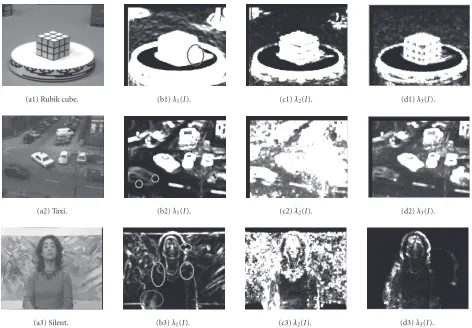
(a1) Rubik cube. (b1)λ1(I). (c1)λ2(I). (d1)λ3(I).
(a2) Taxi. (b2)λ1(I). (c2)λ2(I). (d2)λ3(I).
(a3) Silent. (b3)λ1(I). (c3)λ2(I). (d3)λ3(I).
Figure4: Figures4a1,4a2, and4a3are the 9th frames of the three test sequences; (b), (c), and (d) are the eigenmaps based on the three eigenvaluesλ1,λ2, andλ3, respectively, using conventional fixed-scale 3D structure tensor. Note thatλ1≥λ2≥λ3≥0.
the eigenvalues of local 3D structure tensor can be used to detect the local variances of the input frames.
Thesmallesteigenvalue has been proposed in [9] as the indicator of the frame difference, which was proved to be more robust to noise and low object-background contrast as compared to the simple frame difference. To further in-vestigate, the three eigenmapsbased on the three eigenval-uesλ1(x,y,t),λ2(x,y,t), andλ3(x,y,t) of the local 3D struc-ture tensor are denoted as λ1(I), λ2(I), andλ3(I), respec-tively, and illustrated inFigure 4. It has been observed that, in fact, eigenmap λ1(I) captures both the moving objects and some of isolated texture-like areas in the background. The information revealed in eigenmap λ2(I) as shown in Figures 4c1, 4c2, and 4c3 is not so informative as that of
λ1(I), thus, more difficult to exploit for VO segmentation. Furthermore, eigenmapλ1(I), in general, shows more accu-rate boundaries around the moving VOs and less number of small holes within the VOs’ masks (see Figures4b1,4b2, and
4b3) than those generated byλ3(I) (see Figures4d1,4d2, and
4d3); thus,λ1(I) is selected to generate the motion mask in our scheme.
Notice that both multiple motions (e.g., “Taxi” sequence) and deformable motions (e.g., “Silent” sequence) cannot be
handled accurately by applying the conventional fixed-scale 3D structure tensor. (See Figures 4b2and4b3for demon-stration with explanation provided below.) This is due to the fact that there is no scale adaptation for conventional 3D structure tensor computation. That is, the fixed-scale Σ = [σx σy σt] was used in (2) for the spatio-temporal Gaussian filterH(x,Σ).
Consequently, exploiting large scale size for slow mo-tion will reduce the effectiveness of localization, causing in-accurate motion boundaries as highlighted by the circle in
Figure 4b1. On the other hand, large displacement of a VO cannot be properly matched if a small scale window was ex-ploited, thus, leading to unconnected motion masks as high-lighted by the two small circles inFigure 4b2. Such phenom-ena are also incurred for the deformable moving object as shown inFigure 4b3which contains multiple motions within one body like rotating and translating. Therefore, it is highly desirable to have adaptive scale for the spatio-temporal filter-ing rather than usfilter-ingfixedscale.
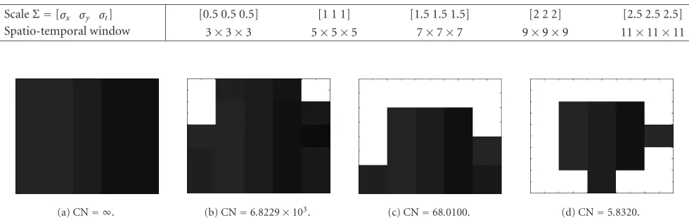
Table1: Experimental scales and spatial windows for the spatio-temporal Gaussian filter, where the three component values inΣcorrespond to the scales on directionsx,y, andt, respectively.
ScaleΣ=[σx σy σt] [0.5 0.5 0.5] [1 1 1] [1.5 1.5 1.5] [2 2 2] [2.5 2.5 2.5]
Spatio-temporal window 3×3×3 5×5×5 7×7×7 9×9×9 11×11×11
(a) CN= ∞. (b) CN=6.8229×10³. (c) CN=68.0100. (d) CN=5.8320.
Figure5: Some typical spatial subregions and their corresponding condition number (CN) computed from the matrix which is constituted by the pixels’ grayvalues: (a) homogeneous region, (b) region with corners, (c) region with edges, and (d) region with corners and edges.
match/capture the motion of a VO with large displacements, thus, leading to unconnected object boundaries. On the other hand, exploiting large scale size for slow motions will reduce the effectiveness of localization and cause blurred mo-tion discontinuities, thus, causing less accurate estimamo-tion due to the local minima. Therefore, representing images at multiple scales is a good approximation of the HVS on per-ceiving images. Several multiscale methods were proposed usingnonlinear filtering[22,23],Gaussian pyramid[5,24], multiwindow[25] orscale-space[26,27,28]. For these mul-tiscale approaches, automatic scale selection is an essential problem to be addressed. Since our method for motion de-tection is based on the 3D structure tensor without dense OF field estimation, we propose an effective automatic scale-selection method with incorporation of the measurement of local image structure.
In the previous works, the spatio-temporal filter with variable scales is introduced in [29] by iterative symmet-ric Schur decomposition. But its scale adaptation through thresholding is determined experimentally. In the 3D struc-ture tensor-based method, the TLS approach [30] is ex-ploited for OF estimation. Since the numerical stability of the TLS solution can be indicated by singular value decom-position (SVD) [30] of the local grayvalue variations, we ex-ploit the condition number to guide the scale selection of the spatio-temporal Gaussian filterH(x,Σ), which is defined as follows. The condition number of a local areaIΩcan be
com-puted by
CondIΩ=IΩIΩ−1=σσmax
min
, (5)
where Ω denotes any area in the input frame whose size is determined by the spatial scales σx andσy of the spatio-temporal filter, which can be referred to inTable 1.σmaxis the maximum singular value andσminis the minimum singular value, which are obtained by performing SVD on the matrix
constituted by the grayvalues of each of the Figures5a,5b,
5c, and5das illustrated. Note that the condition number of a singular matrix is infinite, and a smaller condition number implies a more stable solution.
It can be further observed fromFigure 5that the more homogeneous the area, the larger value the condition num-ber. The reason for this phenomenon is that coherent gray-values will cause high correlation in matrixIΩ; thus, the
com-puted condition number is near to the infinity as shown in
Figure 5a. With the presence of corners and edges, the ma-trix correlation is decreased significantly, and the condition number becomes much smaller (see Figures4b,4c, and4d). Therefore, it is reasonable to use the condition number of the local intensities to steer the scaleΣ of the spatio-temporal Gaussian filter. In our experiments, the initial scaleΣis set to be [0.5 0.5 0.5] (thus, using 3×3×3 window as indi-cated in Table 1), and it will be extended progressively ac-cording toTable 1until either the condition number is below a threshold (e.g., 100) or the scale size reaches the maximum 11×11×11.
The eigenmaps of the largest eigenvalues computed from the scale-adaptive 3D structure tensor are illustrated in
Figure 6. More accurate boundaries and more integrity mo-tion masks can be observed as compared to those inFigure 4
for various test sequences. However, note that the result for thenonrigidmoving VO (seeFigure 6c) fails to yield mean-ingful motion masks. On the contrary, satisfactory motion masks are generated for rigidVOs (see Figures 6aand6b). Thus, a rigidity analysis is developed in the following to dis-tinguish whether the sequence frame contains rigid or non-rigid VOs, and further facilitating the following motion mask generation processes.
4.2.3. Rigidity analysis
(a) Rubik cube. (b) Taxi. (c) Silent.
Figure6: The eigenmapsλ1(I) (the 9th frame) based on thelargesteigenvalues of the scale-adaptive 3D structure tensors.
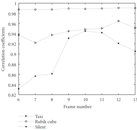
the difference between the motion vectors and the initial-ized velocity. However, its results are affected by the inaccu-racy of VO tracking and motion estimation. Without invok-ing OF computation, we propose an efficient rigidity analysis method by exploiting the correlation between two successive frames based on their 3D structure tensors. The basic concept is quite intuitive as follows. If the moving VO has rigid mo-tion under a certain speed, then only theinterframechanges will be observed. On the other hand, for the nonrigid moving VO, besides the interframe changes, the intraframechanges can also be observed in the body of VOs. Therefore, the cor-relation between two successive frames is expected to be high for rigid VOs and low for nonrigid VOs.
As illustrated in Figures4d1,4d2, and4d3, the eigenmap
λ3(I) inclines to indicate only the moving parts of VOs and reveals much less textured details of the still background than that inλ1(I) (see Figures4b1,4b2, and4b3). Therefore, the correlation coefficientR[32] is computed based on two suc-cessive eigenmaps λ3(It) and λ3(It+1) of framesIt andIt+1, pixels in the frame.
It can be seen that the fluctuation of the curve (see
Figure 7) for rigid VOs (e.g., “Taxi” and “Rubik cube”) is much smoother than that for the nonrigid VO (e.g., “Silent”). Such a fluctuation can be measured by the stan-dard deviation S[32] of the correlation coefficientsRi, for der consideration and ¯Ris the average ofRi. The values ofS computed from “Rubik cube,” “Taxi,” and “Silent,” are 0.013,
1
Figure7: Correlation coefficients computed over a range of succes-sive video frames.
0.0126, and 0.0436, respectively. Based on extensive exper-iments, the threshold for S is determined to be 0.015. Se-quence with the value of Slower than 0.015 is considered having rigid VOs; otherwise, it contains nonrigid VOs.
4.2.4. Motion mask generation and selection
Basics of the eigenvalue analysis of 3D structure tensor
Since tensor-based OF estimation is based on the TLS ap-proach, its solution can be resolved by using the widely used Jacobi method [30] to perform eigenvalue decomposition of the 3D structure tensorJ. The generated three eigenvaluesλk (fork =1, 2, 3), which denote the local grayvalue variations along local dominant directions [17], respectively, can be ex-ploited to derive thecoherency measurementsfor motion field classification.
(a) (b) (c)
Figure8: Maps based on the coherency measurements of the scale-adaptive 3D structure tensors: (a) total coherency measureCt, (b) edge measureCs, and (c) corner measureCc.
(ii) Ifλ1>0 andλ2=λ3=0, that is, rank(J)=1, this in-dicates that the grayvalue changes only happen in the normal direction, indicating that the area contains an edge. This is the well-knownaperture problem encoun-tered in OF estimation.
(iii) Ifλ1 >0,λ2>0, andλ3=0, that is, rank(J)=2, this indicates that a spatio-temporal structure containing grayvalues changes in two directions, and it moves at a constant speed, thus, indicating a corner area. The real motion can be accurately estimated in this case. (iv) If all the three eigenvalues are greater than zero, that is,
rank(J)=3, this indicates that the local area is located on the border of two moving fields under different mo-tions; thus, no reliable motion can be estimated due to the presence of motion discontinuity.
Although the rank ofJproves to contain all necessary in-formation to distinguish different types of motion, it can-not be used for practical implementations because it does not constitute a normalized measure of certainty. Therefore, the coherency measurements for motion field classification have been proposed [17], which yield real-valued numbers between zero and one.
Coherency measurements
The purpose of computing coherency measurements [17] in our method is to provide some indicators regarding the mo-tion of nonrigid moving objects. Instead of using the para-metric approaches for nonrigid VO segmentation as pro-posed in [7,10], which need dense motion field and are sen-sitive to motion estimation errors, anonparametricmethod is proposed here using coherency measurements to quantify the degree of motion estimation certainty. They were derived from the eigenvalues of the 3D structure tensor and can be used as the indicators of local motion structures, such as edge, corner, homogeneous region, and so on. They are de-fined [17] as follows:
(i) total coherency measure:Ct=((λ1−λ3)/(λ1+λ3))2, (ii) edge measure:Cs=((λ1−λ2)/(λ1+λ2))2,
(iii) corner measure:
Cc=Ct−Cs=4 ˙λ1
λ2−λ3
λ2 1−λ2λ3
λ1+λ3 2
λ1+λ2
2 . (8)
The masks of Ct,Cs, andCc computed from the local scale-adaptive 3D structure tensors of “Silent” are illustrated in Figures8a,8b, and8c, respectively. Among them, the map of corner measureCc(i.e.,corner-map) reveals the most dis-tinct VO boundary information to yield the motion masks for nonrigid motions; thus, it is exploited in our framework.
Change detection computation
Change detection is used as the indicator for motion mask selection in our scheme because it can be implemented effi -ciently and enables the detection of appearance motion ac-cording to the predetermined thresholds [33]. The purpose of change detection is to locate moving objects through de-tecting intensity changes between subsequent frames of im-age sequences. One of the change detection techniques is so-calledframe differencingD(N) [33], which is defined as
D(N)=I(t+N)−I(t), (9) where ∗ is theLp norm, andI(t) andI(t+N) are the
tth frame and the (t+N)th frame, respectively. The thresh-old setting ofD(N) depends on the requirement of practical applications. Since the image with noise (e.g., illumination change) may cause false alarms or missing parts of the mo-tion mask, in our method, the threshold forD(N) in (9) is set to be high enough (e.g., 30) in order to avoid the occurrence of false alarm. The missing parts ofD(N) within the areas of moving objects will not affect our motion segmentation re-sults because the final motion masks are not generated from
D(N), it is only used for motion maskselectionhere.
Motion mask selection
(a) (b) (c)
Figure9: Change detection based on the 5th and the 9th frames via (9): (a) “Rubik cube,” rigid rotating motion, (b) “Taxi,” rigid moving VOs under different motions, and (c) “Silent,” nonrigid moving VO.
(a)λ1(I), Rubik cube. (b)λ1(I), Taxi. (c)Cc, Silent.
Figure10: Motion mask selection results (the 9th frame) obtained by the proposed percentage thresholding method using the original motion masks (see Figures6a,6b, and8c) and the corresponding change detection maps (see Figures9a,9b, and9c).
of moving objects correctly from the still background as il-lustrated inFigure 9.
Using a rigid VO as an example, if the size of its mo-tion mask is large enough both in the map D(N) (see Fig-ures9aand9b) and in eigenmapλ1(I) (see Figures6aand
6b), that is, there is distinct motion that occurred within the mask area, thus, the eigenmap mask is considered as part of the moving VO. Otherwise, it is determined to be part of the background. The proposed motion mask selection is per-formed using our proposedpercentage thresholding method as follows.
In order to select (i.e., keep or delete) the masks in eigen-mapλ1(I) one by one, each area (either in white color or in black color inFigure 6) is labeled by an unique number using gray image grass-fire labelingas proposed in [34], which is an extended version of thegrass-fireconcept [35] for gray-level image labeling. The labeled area inλ1(I) is denoted asAeigen. The percentage Rc of change detection maskAchange (white pixels inFigure 9) within the labeled areaAeigenof eigenmap
λ1(I) is computed as
Rc=
Achange
Aeigen ×
100%. (10)
If the value ofRcis larger than the predetermined threshold (e.g., 40 %),Aeigenis kept as the motion mask of a moving VO. Otherwise, areaAeigenis considered as part of the back-ground because there is no distinct motion that occured in it.
For nonrigid motions, the motion mask selection process is implemented in the same way as for rigid motions as
de-scribed above, except that Aeigen should be replaced by the mask Acorner in the corner mapCc (illustrated by the white color in Figure 8c), and the computation of Rc should be modified as
Rc=
Achange
Acorner ×
100%. (11)
After the motion mask selection process, motion masks for moving VOs are generated in eigenmaps (see Figures10a
and10b) and in the corner map (seeFigure 10c), where the homogeneous background and the selected motion masks are shown in black and white colors, respectively.
4.3. Spatial-constrained motion segmentation
However, the motion masks as shown inFigure 10still have small holes in the body of VOs and inaccurate boundaries along the borders of VOs. To address this problem, graph-based image segmentation results (seeFigure 3) as described inSection 4.1is used in order to benefit from the advantages of spatial segmentation, such as the integrity of spatial seg-ments and more accurately segmented boundaries.
(a) Rubik cube. (b) Taxi. (c) Silent.
Figure11: Spatial-constrained motion masks generated based on our method using three video sequences, respectively.
Each spatial segment in the frame illustrated inFigure 3
is labeled by an unique number according to its color. The percentageRmof the motion maskAmaskwithin eachAsegis computed as
Rm=Amask
Aseg ×
100%. (12)
If the value ofRmis larger than the predetermined threshold (e.g., 50 %), the whole spatial segmentAsegshould be viewed as the portion of the moving VO (using white color); oth-erwise, it is treated as part of the background (using black color).
As compared with the motion masks as shown inFigure 10, the spatial-constrained motion masks, as illustrated in Figures 11a, 11b, and 11c, have yielded more accurate boundaries which are aligned with the borders of respective moving VOs. The small holes that occured within some mo-tion masks inFigure 10are also absent inFigure 11.
4.4. Motion-constrained spatial merging
Similar to the synergism existing between the form and mo-tion percepmo-tion pathways in the HVS, the proposed method-ology is to make spatial segmentation and motion estima-tion constrained on each other. For that, the boundary in-formation from image segmentation has contributed to the motion mask generation as described inSection 4.3. On the other hand, how to merge the over-segmented spatial regions based on the motion information is the next issue to be ad-dressed in this section as follows.
There are two classes of region merging approaches: non-parametric techniques [12] and parametric models [10,11]. The nonparametric approach such as boundary melting [12] cannot be integrated with the motion field because the mo-tion field discontinuities are difficult to be identified accu-rately. A parametric method for region merging using en-ergy minimization was proposed in [11] based on Horn’s OF field [36]. The results are sensitive to motion estima-tion errors, and it is computaestima-tionally slow through the it-erative way. Since there is no dense motion field required in our scheme, a novel parametric motion model [10] for the motion-constrained region merging is exploited by using the 3D structure tensor. The parameters of the affine motion model estimated from each spatial segment are used to com-pute the distance between two adjacent segments. Two seg-ments will be merged together if the motion model distance
between them is short enough, that is, sharing the similar motions.
4.4.1. Affine motion model
The planar motion at each pixel positionI(x,y) can be de-scribed by an affine model containing six parameters:
vx(x,y)=ax+by+c,
vy(x,y)=dx+ey+ f,
(13)
wherevxandvyare thexandycomponents of the velocity v, anda,b,c,d,e, andf are the parameters of the model.
The 2D velocity can be extended to 3D directional vec-torvin order to include the unit temporal velocity, which is defined as
The motion-model parameters for a VO are estimated by merging the spatial segmented regions based on a distance function measured between the affine motion model and the 3D structure tensorJi(for pixeli), which can be derived [10] as follows:
dvi,Ji=viTJivi=PTSTiJiSiP=PTQiP, (15) whereQi=STiJiSiis a positive quadratic matrix. The sum of the pixel-wise distances within a given spatial segment con-tainingNpixels is as follows:
Make the partitions ofPandQsegas follows: Now the problem boils down to find the parameters in vector p1 that minimizes dseg(P), and this can be derived as [10] follows:
ˆ
p1= −q−11q2. (19) Thus, the residual distance value is computed by
dseg( ˆP)=qT2pˆ1+g. (20) Notice thatq1 in (19) is not invertible if the spatial seg-ment is (nearly) homogeneous, that is, the vectors inq1are highly correlated. In this case, the estimated parameter is changed to ˆp1 = −q+1q2, whereq+1 is the pseudo inverse of q1. In fact, the invertibility ofq1is not an issue for our ap-plication because the obtained spatial segments contain cer-tain small gradients which can highly decrease the correla-tion among the vectors ofq1.
4.4.3. Normalized distance computation
Since the quadratic form of the velocity in (15) is more sen-sitive to large velocities than to small ones as analyzed in [10], d(vi,Ji) is divided by the norm ofv and the trace of Jito avoid this issue. The normalized distance is defined as follows:
Thus, the normalized residual distance used to measure the motion model distance from each spatial segment to its adjoining segments can be derived from (16) and (20) as fol-lows:
4.4.4. Spatial region merging
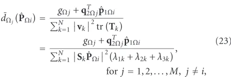
The region merging is implemented based on the parametric motion model described in Section 4.4.2. Firstly, each ment which was obtained from the graph-based image seg-mentation is labeled by a unique number using gray image grass-fire labeling [34]. In each labeled spatial subregionΩi, six affine parameters ˆp1Ωi estimated from (19) are applied to itsM neighborsΩj, for j = 1, 2,. . .,M, but, j = i, to compute thenormalized residue distancefor eachΩj based
on (22):
wherek indicates the sequence number ofN pixels in seg-mentΩj.
If the distance ¯dΩj( ˆPΩi) is below the predetermined threshold, the segmentΩjwill be merged with the segment Ωi to generate a new labeled area. In order to group spa-tial segments into VOs more homogeneously, higher thresh-old (e.g., 0.5) is used for the region merging within the mo-tion masks than the threshold used for the background (e.g., 0.1) because the motion variance in the moving VOs is much higher than that of the background, which is at most caused by the camera motion or illumination changes.
5. EXPERIMENTAL RESULTS
Experimental results for the temporal and the spatial VO seg-mentation are illustrated in Figures 11,12,13, and14, re-spectively. Three kinds of image sequences are chosen for the simulation to show the potential of our method: (1) “Rubik cube,” which contains two rigid rotating objects with simi-lar speeds; (2) “Mother and Daughter,” which involves two objects, one has obvious rotation movement and the other has much less movement; (3) “Taxi,” which has four rigid translational moving objects with different speeds; and (4) “Silent,” which is constituted by a nonrigid moving object in front of a standstill background with complicate textures.
Our spatial-constrained motion masks as illustrated in
Figure 11show that the moving objects can be separated ac-curately from different kinds of background. Both rigid and nonrigid motions can be captured well, using the proposed motion mask generation and selection approaches as de-scribed inSection 4.2. Thanks to the scale-adaptive 3D struc-ture tensor computation, multiple motions are matched cor-rectly as shown in Figure 11b, and notice that even a very small size “walking person” (highlighted by the circle) can also be extracted from the background.
Our spatial-constrained motion segmentation results are also compared with other results obtained from some exist-ing methods [37,38,39,40], as illustrated in Figures12a,
(a1) Ground truth [37]. (a2) Malo’s method [37]. (a3) Our method.
(b1) Altunbasak’s method [38].
(b2) Kim’s method [39]. (b3) Our method.
(c1) Malo’s method [37]. (c2) Bors’s method [40]. (c3) Our method.
Figure12: Segmentedrigidmoving VOs obtained by implementing the motion masks over each original frame of the three test sequences, respectively. The motion masks are yielded either from some existing methods [37,38,39,40] or yielded by our proposed spatial-constrained motion segmentation approach, which have been illustrated inFigure 11as examples.
(a) The 20th frame. (b) The 40th frame. (c) The 60th frame. (d) The 80th frame. (e) The 100th frame. Figure13: Segmentednonrigidmoving VO over several frames of “Silent” sequence.
improved segmentation result on the “walking person” as cir-cled inFigure 12c3, where other approaches failed to capture such a very small-size moving VO. Furthermore, our result yields more accurate boundaries around the taxies as com-pared with Malo’s [37] and Bors’s [40] results as illustrated in Figures 12c1 and12c2, respectively. Notice that the so-claimed ground truth as shown inFigure 12a1is only given as the suggested good segmentation result.
Our motion segmentation results for nonrigid moving VO are presented inFigure 13using several frames of “Silent” sequence as an example. Obviously, our method yields good
VO’s boundary in accordance with human perception, and various motions of the VO have been successfully captured.
Our motion-constrained spatial segmentation results are compared with those proposed in [11] using the same in-put frames as illustrated inFigure 3. Figures14a1,14b1, and
(a1) (b1) (c1)
(a2) (b2) (c2)
Figure14: Motion-constrained spatial segmentation results using graph-based image segmentation (seeFigure 3) as the inputs. Figures
14a1,14b1, and14c1use Ross’s method [11] which is based on Horn’s optical flow [36], and Figures14a2,14b2, and14c2exploit our proposed method which is based on the 3D structure tensor. (a) Rubik Cub. (b) Taxi. (c) Silent.
proposed in [11] was unable to provide the whole back-ground and homogeneous foreback-ground objects. Using our proposed motion-constrained region merging scheme that benefits from the accuracy of spatial-constrained motion mask and the precision of affine motion model-based dis-tance computation, the spatial VOs are segmented correctly from the complex background as illustrated in Figures14a2,
14b2, and14c2.
6. CONCLUSIONS
Using the duality of image and motion segmentations, a new region-based methodology using the 3D structure tensor is developed for extracting not only moving VOs constrained by spatial information, but also spatial VOs constrained by motion information; thus, both the VOs with and without motions can be segmented much more accurately in a unified framework. First, to handle the situation when multiple ob-ject motions occurred in the input image sequence, adaptive scale selection steered by the condition number is exploited for conducting the spatio-temporal Gaussian filtering. Sec-ond, rigidity analysis is performed based on the correlation coefficients of the smallest eigenvalue map computed over a range of successive frames. Third, the largest eigenvalue and the coherency measurements of the 3D structure tensor have been exploited for generating the motion masks of rigid and nonrigid VOs simultaneously. Consequently, the obtained eigenmap and corner map are selected with assistance from the change-detection map, and the boundaries of motion masks are further refined by implementing the spatial con-straint. Fourth, the normalized distance measurement be-tween the affine motion model and the 3D structure
ten-sor is utilized in our scheme to perform motion-constrained spatial region merging via thresholding, in which different thresholds are set for various regions (e.g., moving VOs and the background), respectively. Experimental results show that the performance of our scheme is superior to that of the previous work particularly on the aspects of improving the boundary accuracy of VO segmentation as well as si-multaneously handling multiple VOs with rigid or nonrigid motion.
ACKNOWLEDGMENT
The authors would like to thank the anonymous reviewers for their constructive comments.
REFERENCES
[1] J. Y. A. Wang and E. H. Adelson, “Representing moving im-ages with layers,” IEEE Trans. Image Processing, vol. 3, no. 5, pp. 625–638, 1994.
[2] P. Salembier, F. Marques, M. Pardas, et al., “Segmentation-based video coding system allowing the manipulation of ob-jects,” IEEE Trans. Circuits and Systems for Video Technology, vol. 7, no. 1, pp. 60–74, 1997.
[3] T. Meier and K. N. Ngan, “Automatic segmentation of moving objects for video object plane generation,” IEEE Trans. Cir-cuits and Systems for Video Technology, vol. 8, no. 5, pp. 525– 538, 1998.
[4] J. A. Sethian, Level Set Methods and Fast Marching Methods: Evolving Interfaces in Computational Geometry, Fluid Mechan-ics, Computer Vision, and Materials Science, Cambridge Uni-versity Press, Cambridge, UK, 1999.
segmenta-tion,” inProc. IEEE International Conference on Image Pro-cessing, vol. 2, pp. 73–76, Thessaloniki, Greece, October 2001. [6] M. M. Chang, A. M. Tekalp, and M. I. Sezan, “Simultane-ous motion estimation and segmentation,”IEEE Trans. Image Processing, vol. 6, no. 9, pp. 1326–1333, 1997.
[7] H. Gu, Y. Shirai, and M. Asada, “MDL-based segmentation and motion modeling in a long image sequence of scene with multiple independently moving objects,” IEEE Trans. on Pat-tern Analysis and Machine Intelligence, vol. 18, no. 1, pp. 58– 64, 1996.
[8] M. J. Black and P. Anandan, “The robust estimation of mul-tiple motions: parametric and piecewise-smooth flow fields,”
Computer Vision and Image Understanding, vol. 63, no. 1, pp. 75–104, 1996.
[9] J. Zhang, J. Gao, and W. Liu, “Image sequence segmenta-tion using 3-D structure tensor and curve evolusegmenta-tion,” IEEE Trans. Circuits and Systems for Video Technology, vol. 11, no. 5, pp. 629–641, 2001.
[10] G. Farneback, “Motion-based segmentation of image se-quences,” M.S. thesis, Link¨oping University, Link¨oping, Swe-den, May 1996.
[11] M. G. Ross, “Exploiting texture-motion duality in optical flow and image segmentation,” M.S. thesis, Massachusetts Institute of Technology, Cambridge, Mass, USA, August 2000. [12] M. Sonka, V. Hlavac, and R. Boyle,Image Processing, Analysis,
and Machine Vision, PWS Publishing, Pacific Grove, Calif, USA, 2nd edition, 1999.
[13] S. Ayer and H. S. Sawhney, “Layered representation of motion video using robust maximum likelihood estimation of mix-ture models and MDL encoding,” inProc. 5th International Conference on Computer Vision, pp. 777–784, Boston, Mass, USA, June 1995.
[14] B. A. Wandell, Foundations of Vision, Sinauer Press, Sunder-land, Mass, USA, 1995.
[15] R. M. Haralick and L. G. Shapiro,Computer and Robot Vision, vol. 2, Addison-Wesley, Reading, Mass, USA, 1992.
[16] A. Mitiche and P. Bouthemy, “Computation and analysis of image motion: a synopsis of current problems and methods,”
International Journal of Computer Vision, vol. 19, no. 1, pp. 29–55, 1996.
[17] B. J¨ahne, H. Haussecker, and P. Geissler, Handbook of Com-puter Vision and Applications, vol. 2, pp. 309–396, Academic Press, San Diego, Calif, USA, 1999.
[18] J. L. Barron, D. J. Fleet, and S. S. Beauchemin, “Performance of optical flow techniques,”International Journal of Computer Vision, vol. 12, no. 1, pp. 43–77, 1994.
[19] R. Plankers, “A level set approach to shape recognition,” Tech. Rep., Ecole Polytechnique F´ed´erale de Lausanne, Lausanne, Switzerland, 1997.
[20] P. Felzenszwalb and D. Huttenlocher, “Efficiently computing a good segmentation,” inProc. DARPA Image Understand-ing Workshop, pp. 251–258, Monterey, Calif, USA, November 1998.
[21] I. T. Jolliffe, Principle Component Analysis, Springer-Verlag, New York, NY, USA, 1986.
[22] S. K. Mitra and G. L. Sicuranza, Eds., Nonlinear Image Pro-cessing, Academic Press, San Diego, Calif, USA, 2001. [23] N. U. Ahmed,Linear and Nonlinear Filtering for Scientists and
Engineers, World Scientific, River Edge, NJ, USA, 1998. [24] N. Paragios and G. Tziritas, “Adaptive detection and
localiza-tion of moving objects in image sequences,”Signal Processing: Image Communication, vol. 14, no. 4, pp. 277–296, 1999. [25] F. Bartolini, V. Cappellini, C. Colombo, and A. Mecocci, “A
multiwindow least squares approach to the estimation of op-tical flow with discontinuities,” Optical Engineering, vol. 32, no. 6, pp. 1250–1256, 1993.
[26] K. S. Pedersen and M. Nielsen, “Computing optic flow by scale-space integration of normal flow,” inProc. 3rd Interna-tional Scale-Space Conference, pp. 14–25, Vancouver, British Columbia, Canada, July 2001.
[27] W. J. Niessen, J. S. Duncan, M. Nielsen, L. M. J. Florack, B. M. ter Haar Romeny, and M. A. Viergever, “Multiscale approach to image sequence analysis,”Computer Vision and Image Un-derstanding, vol. 65, no. 2, pp. 259–268, 1997.
[28] M. Gutierrez, M. Rebelo, and S. Furuie, “A multiresolution approach for computing myocardial motion,” inProc. IEEE-SP International Symposium Time-Frequency and Time-Scale Analysis, pp. 89–92, Pittsburgh, Pa, USA, October 1998. [29] M. Middendorf and H.-H. Nagel, “Estimation and
interpreta-tion of discontinuities in optical flow fields,” inProc. 8th IEEE International Conference Computer Vision, vol. 1, pp. 178–183, Vancouver, British Columbia, Canada, July 2001.
[30] G. H. Golub and C. F. Van Loan,Matrix Computations, Jason Hopkins University Press, Baltimore, Md, USA, 1983. [31] A. J. Lipton, “Local application of optic flow to analyze rigid
versus non-rigid motion,” inProc. ICCV Workshop on Frame-Rate Vision, Corfu, Greece, September 1999.
[32] R. J. Larsen and M. L. Marx,An Introduction to Mathematical Statistics and Its Applications, Prentice-Hall, Englewood Cliffs, NJ, USA, 3rd edition, 2001.
[33] T. Aach, A. Kaup, and R. Mester, “Statistical model-based change detection in moving video,”Signal Processing, vol. 31, no. 2, pp. 165–180, 1993.
[34] K.-K Ma and H.-Y. Wang, “Region-based nonparametric op-tical flow segmentation with preclustering and post-clustering,” inProc. International Conference on Multimedia and Expo, vol. 2, pp. 201–204, Lausanne, Switzerland, August 2002.
[35] I. Pitas, Digital Image Processing Algorithms, Prentice-Hall, Englewood Cliffs, NJ, USA, 1993.
[36] B. K. P. Horn and B. G. Schunck, “Determining optical flow,”
Artificial Intelligence, vol. 17, no. 1–3, pp. 185–203, 1981. [37] J. Malo, J. Gutierrez, I. Epifanio, and F. J. Ferri,
“Perceptu-ally weighted optical flow for motion-based segmentation in MPEG-4 paradigm,” Electronics Letters, vol. 36, no. 20, pp. 1693–1694, 2000.
[38] Y. Altunbasak, P. E. Eren, and A. M. Tekalp, “Region-based parametric motion segmentation using color information,”
Journal of Graphical Models and Image Processing, vol. 60, no. 1, pp. 13–23, 1998.
[39] M. Kim, J. G. Choi, D. Kim, et al., “A VOP generation tool: au-tomatic segmentation of moving objects in image sequences based on spatio-temporal information,” IEEE Trans. Circuits and Systems for Video Technology, vol. 9, no. 8, pp. 1216–1226, 1999.
[40] A. G. Bors and I. Pitas, “Optical flow estimation and mov-ing object segmentation based on median radial basis func-tion network,”IEEE Trans. Image Processing, vol. 7, no. 5, pp. 693–702, 1998.
Kai-Kuang Ma received the Ph.D. degree from North Carolina State University, and the M.S. degree from Duke University, USA, both in electrical engineering, and the B.E. degree from Chung Yuan Christian Uni-versity, Taiwan, in electronic engineering. He is a tenured Associate Professor in the School of Electrical and Electronic Engi-neering, Nanyang Technological University, Singapore. His research interests are in the