A Measure of Term Representativeness Based on the Number of Co occurring Salient Words

A Measure of Term Representativeness Based on the Number of

Co-occurring Salient Words

Toru Hisamitsu and Yoshiki Niwa

Central Research Laboratory, Hitachi, Ltd. Hatoyama, Saitama, 350-0095, Japan {hisamitu, yniwa}@harl.hitachi.co.jp

Abstract

We propose a novel measure of the representativeness (i.e., indicativeness or topic specificity) of a term in a given corpus. The measure embodies the idea that the distribution of words co-occurring with a representative term should be biased according to the word distribution in the whole corpus. The bias of the word distribution in the co-occurring words is defined as the number of distinct words whose occurrences are saliently biased in the co-occurring words. The saliency of a word is defined by a threshold probability that can be automatically defined using the whole corpus. Comparative evaluation clarified that the measure is clearly superior to conventional measures in finding topic-specific words in the newspaper archives of different sizes.

Introduction

Measuring the representativeness (i.e., the informativeness or domain specificity) of a term１ is

essential to various tasks in natural language processing (NLP) and information retrieval (IR). Such a measure is particularly crucial to automatic dictionary construction and IR interfaces to show a user words indicative of topics in retrievals that often consist of an intractably large number of documents (Niwa et al. 2000).

This paper proposes a novel and effective measure of term representativeness that reflects the bias of the words co-occurring with a term. In the following, we focus on extracting topic words from an archive of newspaper articles.

In the literature of NLP and IR, there have been a number of studies on term weighting, and these are strongly related to measures of term

１ _{A term is a word or a word sequence.}

representativeness (see section 1). In this paper we employ the basic idea of the ‘baseline method’ proposed by Hisamitsu (Hisamitsu et al. 2000). The idea is that the distribution of words co-occurring with a representative term should be biased according to the word distribution of the whole corpus. Concretely, for any term T and any measure

M for the degree of bias of word occurrences in

D(T), a set of words co-occurring with T, according to those of the whole corpus D0, the baseline method

defines representativeness of term T by normalizing M(D(T)). In what follows, D0 is an archive of

newspaper articles and D(T) is defined as the set of all articles containing T.

The normalization of M(D(T)) is done by a function BM, called the baseline function, which

estimates the value of M(Drand) using #Drand for any

randomly sampled document (in our case, ‘article’) set Drand, where #Drand stands for the total number of

words contained in Drand. By dividing M(D(T)) by

BM(#D(T)), comparison of M(D(T1)) and M(D(T2))

becomes meaningful even if the frequencies of T1

and T2 are very different. We denote this normalized

value by NormM(D(T)).

Hisamitsu et al. reported that NormM(D(T)) is very effective in capturing topic-specific words when M(D(T)) is defined as the distance between two word distributions PD(T) and P0 (see subsection

1.2), which we denote by Dist(D(T)).

Although NormDist(D(T)) outperforms existing measures, it has still an intrinsic drawback shared by other measures, that is, words which are irrelevant to

T and simply happen to occur in D(T) --- let us call these words non-typical words --- contribute to the calculation of M(D(T)). Their contribution accumulates as background noise in M(D(T)), which is the part to be offset by the baseline function. In other words, if M(D(T)) were to exclude the contribution of non-typical words, it would not need to be normalized and would be more precise.

a discrete way: that is, we only take words whose occurrences are salientlybiased in D(T) into account, and let the number of such words be the degree of bias of word occurrences in D(T). Thus, SAL(D(T),

s), the number of words in D(T) whose saliency is over a threshold value s, is expected to be free from

the background noise and sensitive to number of

major subtopics in D(T). The essential problem now is how to define the saliency of bias of word occurrences and the threshold value of saliency. This paper solves this problem by giving a mathematically sound measure. Furthermore, it is shown that the optimal threshold value can be defined automatically. The newly defined measure

SAL(D(T), s) outperforms existing measures in picking out topic-specific words from newspaper articles.

1. Brief review of term representativeness

measures

1.1 Conventional measures

Regarding term weighting, various measures of importance or domain specificity of a term have been proposed in NLP and IR domains (Kageura et al. 1996). In his survey, Kageura introduced two aspects of a term: unithood and termhood. Unithood is "the degree of strength or stability of syntagmatic combinations or collocations," and termhood is "the degree to which a linguistic unit is related to (or more straightforwardly, represents) domain-specific concepts." Kageura's termhood is therefore what we call representativeness here.

Representativeness measures were first introduced in the context of determining indexing words for IR (for instance, Salton et al. 1973; Spark-Jones et al. 1973; Nagao et al. 1976). Among a number of measures introduced there, the most commonly used one is tf-idf proposed by Salton et al. There are a variety of modifications of tf-idf (for example, Singhal et al. 1996) but all share the basic feature that a word appearing more frequently in fewer documents is assigned a higher value.

In NLP domains several measures concentrating on the unithood of a word sequence have been proposed. For instance, the mutual information (Church et al. 1990) and log-likelihood ratio (Dunning 1993; Cohen 1995) have been widely used for extracting word bigrams. Some measures for termhood have also been proposed, such as Imp

(Nakagawa 2000), C-value and NC-value (Mima et

al. 2000).

Although certain existing measures are widely used, they have major problems as follows: (1) classical measures such as tf-idf are so sensitive to term frequencies that they fail to avoid uninformative words that occur very frequently; (2) measures based on unithood cannot handle single-word terms; and (3) the threshold value for a term to be considered as being representative is difficult to define or can only be defined in an ad hoc manner. It is reported that measures defined by the baseline method do not have these problems (Hisamitsu et al. 2000).

1.2 Baseline method

The basic idea of the baseline method stated in

introduction can be summarized by the famous

quote (Firth 1957) :

"You shall know a word by the company it keeps." This is interpreted as the following hypothesis:

For any term T, if the term is

representative, word occurrences in

D(T), the set of words co-occurring with T, should be biased according to the word distribution in D0.

This hypothesis is transformed into the following procedure:

Given a measure M for the bias of

word occurrences in D(T) and a term

T, calculate M(D(T)), the value of the measure for D(T). Then compare

M(D(T)) with BM(#D(T)), where #D(T) is the number of words contained in #D(T), and BM estimates the value of M(D) when D is a randomly chosen document set of size #D(T).

Here, as stated in introduction, D(T) is considered to be the set of all articles containing term T.

Hisamitsu et al. tried a number of measures for

M, and found that using Dist(D(T)), the distance between the word distribution PD(T) in D(T) and the

word distribution P0 in the whole corpus D0 is

effective in picking out topic-specific words in newspaper articles. The value of Dist(D(T)) can be defined in various ways, and they found that using log-likelihood ratio (see Dunning 1993) worked best which is represented as follows:

0

# log )

( # log

D K k T D

k

k M i

i i

i i

M

i i

i

∑

∑

= =

− ,

D(W) and D0 respectively, and {w1,...,wM} is the set

of all words in D0.

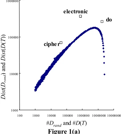
As stated in introduction, Dist(D(T)) is normalized by the baseline function, which is referred as BDist(•) here. Figure 1(a) illustrates the

necessity of the normalization: the graph’s coordinates are {(#D(T), Dist(D(T))) and {(#Drand,

Dist(Drand))}, where T varies over “cipher”, “do”,

and “economy”, and Drand varies over a wide

numerical range of randomly sampled articles. This figure shows that Dist(D(“do”)) is smaller than

Dist(D(“electronic”)), which reflects our linguistic intuition that words co-occurring with “electronic” are more biased than those with “do”. However,

Dist(D(“cipher”)) is smaller than Dist(D(“do”)), which contradicts our linguistic intuition. This is why values of Dist(D(T)) are not directly used to compare the representativeness of terms.

Figure 1(a)

Baseline curve and sample word distribution

This phenomenon can be explained by the curve, referred to as the baseline curve, composed of {(#Drand, Dist(Drand)}. The curve indicates that a part

of Dist(D(T)) systematically varies depending only on #D(T) and not on T itself. It indicates the very notion of background noise stated in introduction, and by offsetting this part using the baseline function BDist(#D(T)), which approximates the

baseline curve, the graph is converted into that of Figure 1(b). Since the baseline curve is not very meaningful as #Drand approaches to #D0, extremely

frequent terms, such as “do” are treated in a special way: that is, if the number of documents in D(T) is larger than a threshold value N0, which was

calculated from the average number of words contained in a document, N0 documents are

randomly chosen from D(T). This is because the

coordinates of the point corresponding to “do” differ in Fig. 1(a) and Fig. 1(b). As stated in introduction, Hisamitsu et al. (2000) reported on that the superiority of NormDist(D(T)), normalized

Dist(D(T)), in picking out topic-specific words over various measures including existing ones and other ones developed by using the baseline method.

Figure 1(b) Effect of Normalization

1.3 Reconsideration of normalization

The effectiveness of the baseline method’s normalization indicates that Dist(D(T)) can be decomposed into two parts, one depending on T

itself and another depending only on the size of D(T), which is considered to be background noise. The essence of the baseline method is to make the

background noise explicit as a baseline function and to offset the noise by using the baseline function. To put it the other way round, if a term representativeness measure is designed so that this noise part does not exist in the first place, there is no need for the baseline function and calculation of representativeness becomes much simpler. More importantly, the precision of the measure itself should improve.

The definition of Dist(D(T)) shows, as with other measures, that every word in D(T) contributes to the value of Dist(D(T)). This explains why

background noise, BDist(#D(T)), grows as #D(T)

increases. One way to improve this situation is to eliminate the contribution of non-typical (see

introduction) words. The simplest way to archive

this is to focus only on saliently occurring words (precisely, words whose occurrences are saliently biased in D(T)) and let the number of words whose saliency is over a threshold value s, denoted by

SAL(D(T), s), be the degree of bias of word

1000 10000 100000 1000000

100 1000 10000 100000 1000000 10000000 100000000

ciphe r

100 1000 10000 100000 1000000 10000000 100000000

ciphe r

0 5000 10000 15000 20000 25000 30000 35000 40000 45000 50000

cipher

0 5000 10000 15000 20000 25000 30000 35000 40000 45000 50000

occurrences in D(T). SAL(D(T), s) should reflect the richness of subtopics in D(T) and should be free from the contribution of non-typical words in D(T).

Thus, we need to define the saliency of

occurrences of a word and a threshold value with

which the occurrences of a word in D(T) is determined as salient.

2. Term representativeness measure based on

the number of co-occurring salient words

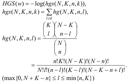
2.1 A measure of word occurrence saliency

To define saliency of occurrences of a word w in

D(T), we employ a probabilistic measure proposed by Hisamitsu et al. (2001) as follows:

Let the total number (occurrences) of words in the whole corpus be N, the number (occurrences) of words in D(T) be n, the frequency of w in the whole corpus be K, and the frequency of w in

D(T) be k. Denote the probability of “No less than k red balls are contained in n balls that are arbitrarily chosen from N balls containing K red balls” by hgs(N, K, n, k). Then the saliency of w

in D(T) is defined as −log(hgs(N, K, n, k))２.

Note that the probability of “k red balls are contained in n balls arbitrarily chosen from N balls containing K red balls”, which we denote as hg(N, K,

n, k), is a hypergeometric distribution with variable

k. We denote the value −log(hgs(N, K, n, k)) by

Due to its probabilistic meaning, comparison of the

２ _{The reason why HGS(v) should be defined by} −_hgs(N, K, n, k) instead of −hg(N, K, n, k) is that the value of −hg(N, K, n, k) itself cannot tell whether occurrence of v k-times is saliently frequent or saliently infrequent. Only

hgs(N, K, n, l), the sum of hg (N, K, n, l) over l

k. HGS(w) can be calculated very efficiently using an approximation technique (Hisamitsu et al. 2001).

2.2 Definition of SAL(D(T), s)

Now we can define SAL(D(T), s) using the saliency occurrence is not less than s. For instance, using the 1996 archive of Nihon Keizai Shimbun (a Japanese financial newspaper), SAL(D(“Aum３”), 110) = 74,

SAL(D(“Aum”), 200) = 50, SAL(D*(“do”), 110) = 1, and SAL(D*(“do”), 200) = 0, where D*(“do”) is a set of N0 randomly chosen articles from D(“do”) and

N0 is the threshold value stated in subsection 1.2.

This strongly suggests that SAL(D(T), s) can discriminate topic-specific words from non-topical words.

2.3 Optimizing threshold of saliency

Note that SAL(D(T), 0) gives the number of distinct words in D(T), and as s increases to ∞, SAL(D(T), s) becomes a constant function (zero). If we straightforwardly follow the baseline method, we have to construct the baseline function BSAL(D(T), s) for

varying s and test the performance of

NormSAL(D(T), s), the normalized SAL(D(T), s). There are, however, a problem that BSAL(D(T), s) cannot

be precisely approximated because SAL(D(T), s) is a discrete-valued function.

By considering the meaning of the baseline function, we can solve the problem of determining the optimal value of saliency parameter s without approximating baseline functions. That is, since the baseline function is considered as background noise

to be offset, the best situation should be that the baseline function is a constant-valued function while

SAL(D(T), s) is a non-trivial function (i.e., not a constant function). If there exists s0 satisfying the

condition, SAL(D(T), s0) does not need to be

normalized and is reliable itself, and s0 is the optimal

parameter.

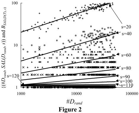
Figure 2 plots the coordinates {#Drand,

３ _{Aum is the name of a religious cult that attacked Tokyo}

SAL(Drand, s)} for Drand and s, where Drand varies

over randomly sampled article sets and s varies over several discrete values. Although BSAL(D(T), s) cannot

be precisely approximated by using analytical functions, it can be seen that BSAL(D(T), s) changes from

a monotone increasing function to a monotone decreasing function when s is greater than about 110, and the graph of BSAL(D(T), 110) is roughly parallel to

the x-axis. Considering the meaning of baseline functions again, this means that s0 = 110 is the

optimal value of saliency and that SAL(D(T), 110) can be used without normalization and is the most effective SAL. The important thing here is that this procedure to find the optimal value of s can be done automatically because it only requires random sampling of documents and curve fitting. Section 3 experimentally confirms the superiority of SAL(D(T),

s0) as a representativeness measure.

Figure 2

{(#Drand, SAL(Drand, s)) and BSAL(D(T), s)

3. Experiments

As in Hisamitsu et al. (2000), taking topic-word selection for IR navigation into account, we examined the relation between the value of representative measures and a manual classification of words (monograms) extracted from nearly 160,000 articles in the 1996 archive of the Nihon Keizai Shimbun (denoted by D0 later on).

3.1 Preparation

We randomly chose 20,000 words from 86,000 words having document frequencies larger than 2 in

D0, then randomly chose 2,000 of them and

classified these into three groups: (1) class P

(positive): topic-specific words which are useful for the navigation of IR, (2) class N (negative): words,

such as “do”, not topic-specific and useless for IR navigation, and (3) class U (uncertain): words whose usefulness in IR navigation was either neutral or difficult to judge. In the classification process, a judge used an IR system called DualNAVI (Niwa et al. 2000) having dual windows one of which shows the titles of retrieved articles and another displays salient words occurring in the articles. The details of the guideline of classification are stated in Hisamitsu et al. (2001).

3.2 Measures compared in the experiments

Four measures were compared by Hisamitsu et al. (2000): NormDist(D(T)), NormDIFFNUM(D(T)),

tf-idf, and tf(term frequency), where

NormDIFFNUM(D(T)) is a normalized version of a

measure called DIFFNUM(D(T)), which gives the number of distinct words in D(T). DIFFNUM is based on the hypothesis that the number of distinct words co-occurring with a representative word is smaller than that with a generic word (Teramoto et al. 1999). The definition of tf-idf used in the comparison was as follows:

, ) ( log ) (

T N N T

TF idf

tf _{− = ×} total

where T is a term, TF(T) is the term frequency of T,

Ntotal is the total number of documents, and N(T) is

the number of documents that contain T. We compared these four measures with SAL(D(T), s), varying s.

3.3 Comparative experiments and results

We compared the ability of each measure to gather class P words. We randomly sorted the 20,000 words mentioned above, and then compared the result with the results of sorting by other measures. The comparison was done using the accumulated number of words marked by class P that appeared in the first k (1 ≤ k≤ 20,000) words. For simplicity, we use the following notation:

Rand(P, k): the accumulated number of class P

words appearing in the first k words when random sorting was applied,

M(P, k): the accumulated number of class P

words appearing in the first k words when sorting was done by measure M,

DP(M, k) = M(P, k)- Rand(P, k), and

.) , ( )

, (

1

∑

=

= k

l

l M DP k

M ADP

The values of DP(M, k) and ADP(M, k) are called

1 10 100

1000 10000 100000

s=20 s=40

s=120

s=110 s=100 s=80 s=60

s=90

#Drand

{(#

Drand

,

SAL

(

Drand

,

s

)) and

BSAL

(

D

(

T

),

s

DP-score and ADP-score, respectively. For these scores, higher is better.

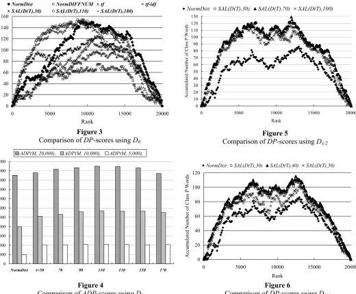
Figure 3 compares DP(M, k) for 1 ≤ k≤ 20,000 and Figure 4 compares ADP(M, 5,000), ADP(M,

10,000), and ADP(M, 20,000). Where M varies over {NormDist(D(•)), NormDIFFNUM(D(•)), tf-idf, tf,

SAL(D(•), s)}. These figures shows that SAL(D(T),

s0) is overall superior to other measures except

NormDist(D(•)). It is also superior to

NormDist(D(•)) for 0≤k≤15,000. In terms of

ADP-scores, SAL(D(T), s0) is superior to all other

measures for k=5,000，10,000, 20,000. This means that SAL(D(•), s0) is superior to NormDist(D(•)) on

the whole, and particularly superior in gathering topic-specific words near the top of the sorting. Comparison of SAL(D(T), s) for different values of s

shows that s = s0 is actually the optimal value.

3.4 Effect of corpus size

To see the effect of corpus size on the

performance of

SAL

(

D

(

•

),

s

), we conducted the

same kind of experiments that compared

NormDist

(

D

(

•)

) and

SAL

(

D

(

•

),

s

) by using

different size of corpora

D

and

D

, whose

sizes were 1/2 and 1/4 of

D

respectively. The

optimal value of

s

was determined for each

corpus in the same way as stated in subsection

2.3. The optimal value was around 70 for

D

and around 40 for

D

. Figure 5 compares

DP

-scores when

D

is used. Figure 6 compares

the same when

D

is used. Figures 5 and 6

show that

SAL

(

D

(

•

),

s

) is superior to

NormDist

(

D

(

•)

) for corpora of different sizes.

Judging from the results, we expect that the

superiority of

SAL

(

D

(

•

),

s

) would be even

more apparent for a larger corpus.

0 10 20 30 40 50 60 70 80 90 100 110 120 130

0 5000 10000 15000 20000 Rank

Accum

ulated

Num

ber of

Class P Word

s

NormDist SAL(D(T),30) SAL(D(T),70) SAL(D(T),100)

0 20 40 60 80 100 120

0 5000 10000 15000 20000

Rank

Acc

um

ula

ted Num

be

r of Class P

Words

NormDist SAL(D(T),30) SAL(D(T),40) SAL(D(T),50)

Figure 4

Comparison of ADP-scores using D0

Figure 3

Comparison of DP-scores using D0

Figure 5

Comparison of DP-scores using D1/2

Figure 6

Comparison of DP-scores using D1/4

0 2000 4000 6000 8000 10000 12000 14000 16000 18000 20000 22000

NormDist s=50 70 90 110 130 150 170

AD

P-score

ADP(M, 20,000), ADP(M, 10,000), ADP(M, 5,000),

0 20 40 60 80 100 120 140 160

0 5000 10000 15000 20000

Rank

A

ccu

m

ula

ted

N

um

ber o

f Class

P W

ord

s

NormDist NormDIFFNUM tf tf-idf

Conclusion

We proposed a novel measure of the representativeness of a term T in a given corpus. Denoting the words co-occurring with T by D(T), the measure is defined as SAL(D(T), s), the number of words in D(T) whose saliency of occurrences is over a threshold s. This measure embodies the idea that the distribution of words in D(T) should be saliently biased according to that of the whole corpus if T is a representative term. The saliency of word occurrences is defined by using a combinatorial probability, and the threshold value s

is defined automatically so that the baseline function of SAL(D(T), s) does not depend on #D(T), the number of words contained in D(T). Comparative evaluation clarified that the proposed measure is superior to conventional measures in finding topic-specific words in newspaper archives of different sizes.

Acknowledgements

We would like to express our gratitude to Prof. Jun-ichi Tsujii of the University Tokyo and Prof. Kyo Kageura of National Institute of Informatics for their insightful comments.

This project is supported in part by the Core Research for Evolutional Science and Technology (CREST) under the auspices of the Japan Science and Technology Corporation.

References

Church, K. W. and Hanks, P. (1990). Word Association Norms, Mutual Information, and Lexicography,

Computational Linguistics 6(1), pp.22-29.

Cohen, J. D. (1995). Highlights: Language- and

Domain-independent Automatic Indexing Terms for Abstracting, Journal of American Soc. for Information

Science 46(3), pp.162-174.

Dunning, T. (1993). Accurate Method for the Statistics of Surprise and Coincidence, Computational Linguistics 19(1), pp.61-74.

Firth, J. A synopsis of linguistic theory 1930-1955. (1957). Studies in Linguistic Analysis, Philological Society, Oxford.

Hisamitsu, T., Niwa, Y., and Tsujii, J. (2000). A Method of Measuring Term Representativeness - Baseline Method Using Co-occurrence Distribution-, Proc. of

COLING2000, pp.320-326.

Hisamitsu, T., Niwa, Y. (2001). Topic-Word Selection

Based on Combinatorial Probability, Proc. of

NLPRS2001, pp.289-296.

Kageura, K. and Umino, B. (1996). Methods of automatic

term recognition: A review. Terminology 3(2),

pp.259-289.

Mima, H. and Ananiadou, S. (2000). An application and e aluation of the C/NC-value approach for the automatic term recognition of multi-word units in Japanese,

Terminology, Vol.6, No.2, pp. 175–194.

Nagao, M., Mizutani, M., and Ikeda, H. (1976). An Auto- mated Method of the Extraction of Important Words from Japanese Scientific Documents, Trans. of IPSJ, 17(2), pp.110-117.

Nakagawa, H. (2000). Automatic Term Recognition based on Statistics of Compound Nouns", Terminology, Vol.6, No.2, pp.195 – 210.

Niwa, Y., Iwayama, M., Hisamitsu, T., Nishioka, S., Takano, A., Sakurai, H., and Imaichi, O.(2000).

DualNAVI -dual view interface bridges dual query

types, Proc. of RIAO 2000, pp.19-20.

Salton, G. and Yang, C. S. (1973). On the Specification of

Term Values in Automatic Indexing. Journal of

Documentation 29(4), pp.351-372.

Singhal, A., Buckley, C., and Mitra, M. (1996). Pivoted Document Length Normalization, Proc. of ACM SIGIR’ 96, pp.21-29.

Sparck-Jones, K. (1973). Index Term Weighting.

Information Storage and Retrieval 9(11), pp.616-633.

Teramoto, Y., Miyahara, Y., and Matsumoto, S. (1999). Word weight calculation for document retrieval by

analyzing the distribution of co-occurrence words, Proc.